from lxml.html import parse
from urllib.request import urlopen
from pandas.io.parsers import TextParser
import pandas as pd
from pandas import DataFrame, Series
import folium
import numpy as np
# we are using the inline backend
%matplotlib inline

import matplotlib as mpl
import matplotlib.pyplot as plt
Prepare the data
Getting data from ministry of health
basepath = os.getcwd() # get the location of current .py file
The excel file(‘covid-caselist-23april.xlsx’) is from the Ministry of Health website on 23/04/2020.
filename= os.path.join(basepath,'covid-caselist-23april.xlsx')
df = pd.read_excel(filepath, sheet_name='Confirmed')
df.head() # preview of the data
|
Date of report |
Sex |
Age group |
DHB |
Overseas travel |
Last country before return |
Flight number |
Flight departure date |
Arrival date |
| 0 |
22/04/2020 |
Female |
20 to 29 |
Counties Manukau |
No |
NaN |
NaN |
NaT |
NaT |
| 1 |
22/04/2020 |
Male |
40 to 49 |
Hawke's Bay |
No |
NaN |
NaN |
NaT |
NaT |
| 2 |
21/04/2020 |
Female |
70+ |
Waikato |
|
NaN |
NaN |
NaT |
NaT |
| 3 |
19/04/2020 |
Female |
30 to 39 |
Bay of Plenty |
|
NaN |
NaN |
NaT |
NaT |
| 4 |
19/04/2020 |
Male |
50 to 59 |
Bay of Plenty |
No |
NaN |
NaN |
NaT |
NaT |
Treating the raw data
Use followed function to change to type of the data.
df['Age group'] = df['Age group'].astype('str')
df['Age group'].duplicated(keep='first')
0       False
1       False
2       False
3       False
4       False
        ...
1446     True
1447     True
1448     True
1449     True
1450     True
Name: Age group, Length: 1451, dtype: bool
df.head()
|
Date of report |
Sex |
Age group |
DHB |
Overseas travel |
Last country before return |
Flight number |
Flight departure date |
Arrival date |
| 0 |
22/04/2020 |
Female |
20 to 29 |
Counties Manukau |
No |
NaN |
NaN |
NaT |
NaT |
| 1 |
22/04/2020 |
Male |
40 to 49 |
Hawke's Bay |
No |
NaN |
NaN |
NaT |
NaT |
| 2 |
21/04/2020 |
Female |
70+ |
Waikato |
|
NaN |
NaN |
NaT |
NaT |
| 3 |
19/04/2020 |
Female |
30 to 39 |
Bay of Plenty |
|
NaN |
NaN |
NaT |
NaT |
| 4 |
19/04/2020 |
Male |
50 to 59 |
Bay of Plenty |
No |
NaN |
NaN |
NaT |
NaT |
#replace the emply values with 'Unknown'
df.replace(to_replace=r'^\s*$',value='Unknown',regex=True,inplace=True)
#replace the space in the columns name to avoid potential problems
df.columns = list(i.replace(' ','_') for i in df.columns)
df.columns
Index(['Date_of_report', 'Sex', 'Age_group', 'DHB', 'Overseas_travel',
       'Last_country_before_return', 'Flight_number', 'Flight_departure_date',
       'Arrival_date'],
      dtype='object')
df = df.rename(columns = {'Date_of_report':'Report_Date','Overseas_travel':'Overseas','Age_Group':'Age_group'})
df =df.iloc[:,:6]
df.head()
|
Report_Date |
Sex |
Age_group |
DHB |
Overseas |
Last_country_before_return |
| 0 |
22/04/2020 |
Female |
20 to 29 |
Counties Manukau |
No |
NaN |
| 1 |
22/04/2020 |
Male |
40 to 49 |
Hawke's Bay |
No |
NaN |
| 2 |
21/04/2020 |
Female |
70+ |
Waikato |
Unknown |
NaN |
| 3 |
19/04/2020 |
Female |
30 to 39 |
Bay of Plenty |
Unknown |
NaN |
| 4 |
19/04/2020 |
Male |
50 to 59 |
Bay of Plenty |
No |
NaN |
df['Report_Date'] =pd.to_datetime(df['Report_Date'],format='%d/%m/%Y')
df.sort_values(by ='Report_Date', axis=0, inplace= True )
df.head()
|
Report_Date |
Sex |
Age_group |
DHB |
Overseas |
Last_country_before_return |
| 1111 |
2020-02-26 |
Female |
60 to 69 |
Auckland |
Yes |
Indonesia |
| 1110 |
2020-03-02 |
Female |
30 to 39 |
Waitemata |
Yes |
Singapore |
| 1108 |
2020-03-04 |
Male |
40 to 49 |
Counties Manukau |
No |
NaN |
| 1109 |
2020-03-04 |
Male |
40 to 49 |
Waitemata |
Yes |
Singapore |
| 1450 |
2020-03-05 |
Female |
70+ |
Waitemata |
Yes |
United States of America |
Preparing the plotting data
Group data by DHB
df2=df.groupby('DHB').count()
df2.head(2)
|
Report_Date |
Sex |
Age_group |
Overseas |
Last_country_before_return |
| DHB |
|
|
|
|
|
| Auckland |
186 |
186 |
186 |
186 |
75 |
| Bay of Plenty |
47 |
47 |
47 |
47 |
21 |
df_DHB = df2.iloc[:,1]
df_DHB.head()
DHB
Auckland             186
Bay of Plenty         47
Canterbury           157
Capital and Coast     95
Counties Manukau     111
Name: Sex, dtype: int64
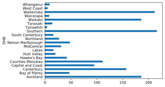
df_DHB.plot.barh() #directly plot to have a general view
<matplotlib.axes._subplots.AxesSubplot at 0x23c3c861048>
Group data by age
df_age = df.groupby('Age_group').count()
df_age = df_age.iloc[:,1]
df_age.head(2)
Age_group
1 to 4      17
10 to 14    40
Name: Sex, dtype: int64
df_age.sum()
1450
Group data by gender
df_gender = df.groupby('Sex').count()
df_gender = df_gender.iloc[:,1]
df_gender.head()
Sex
Female    802
Male      648
Name: Age_group, dtype: int64
Group data according to the case detail
df.head(2)
|
Report_Date |
Sex |
Age_group |
DHB |
Overseas |
Last_country_before_return |
| 1111 |
2020-02-26 |
Female |
60 to 69 |
Auckland |
Yes |
Indonesia |
| 1110 |
2020-03-02 |
Female |
30 to 39 |
Waitemata |
Yes |
Singapore |
df_info = df.groupby('Overseas').count()
df_info = df_info.iloc[:,1]
df_info.head()
Overseas
No         833
Unknown     56
Yes        561
Name: Sex, dtype: int64
Group data by Last_City_before_NZ
df_city= df.groupby('Last_country_before_return').count().sort_values(by = 'Overseas')
df_city.head()
|
Report_Date |
Sex |
Age_group |
DHB |
Overseas |
| Last_country_before_return |
|
|
|
|
|
| Vietnam |
1 |
1 |
1 |
1 |
1 |
| Middle East |
1 |
1 |
1 |
1 |
1 |
| Mexico |
1 |
1 |
1 |
1 |
1 |
| Uruguay |
1 |
1 |
1 |
1 |
1 |
| Portugal |
1 |
1 |
1 |
1 |
1 |
df100 = df_city.iloc[:,-1]
df_city = df100[-6:-1]
df_city
Last_country_before_return
Singapore               26
Qatar                   36
United Kingdom          59
United Arab Emirates    69
Australia               98
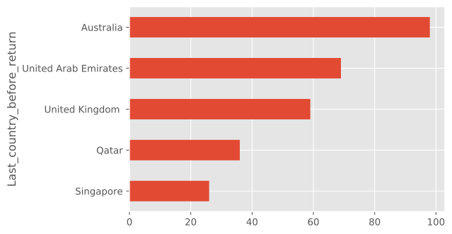
Name: Overseas, dtype: int64
df_city.name
'Overseas'
df_city.index.name
'Last_country_before_return'
df_city.index.Name = 'Last_country_before_return'
df_city
Last_country_before_return
Singapore               26
Qatar                   36
United Kingdom          59
United Arab Emirates    69
Australia               98
Name: Overseas, dtype: int64
print(plt.style.available)
mpl.style.use(['ggplot']) # optional: for ggplot-like style
['bmh', 'classic', 'dark_background', 'fast', 'fivethirtyeight', 'ggplot', 'grayscale', 'seaborn-bright', 'seaborn-colorblind', 'seaborn-dark-palette', 'seaborn-dark', 'seaborn-darkgrid', 'seaborn-deep', 'seaborn-muted', 'seaborn-notebook', 'seaborn-paper', 'seaborn-pastel', 'seaborn-poster', 'seaborn-talk', 'seaborn-ticks', 'seaborn-white', 'seaborn-whitegrid', 'seaborn', 'Solarize_Light2', 'tableau-colorblind10', '_classic_test']
dfList = [df_DHB, df_age, df_gender, df_info,df_city]
df_city.plot.barh() # bar plot
<matplotlib.axes._subplots.AxesSubplot at 0x23c3d903388>
df_city.index.name = 'Last_country_before_return'
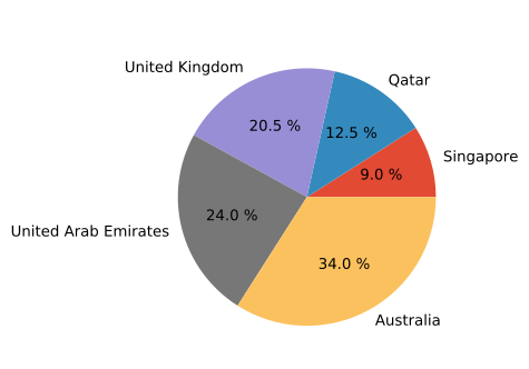
df_city.plot.pie(x=df_city.values, labels=df_city.index, autopct='%3.1f %%', title = df_city.name) # pie plot
<matplotlib.axes._subplots.AxesSubplot at 0x23c3d999a48>
Plotting
Define a vertical bar plotting function
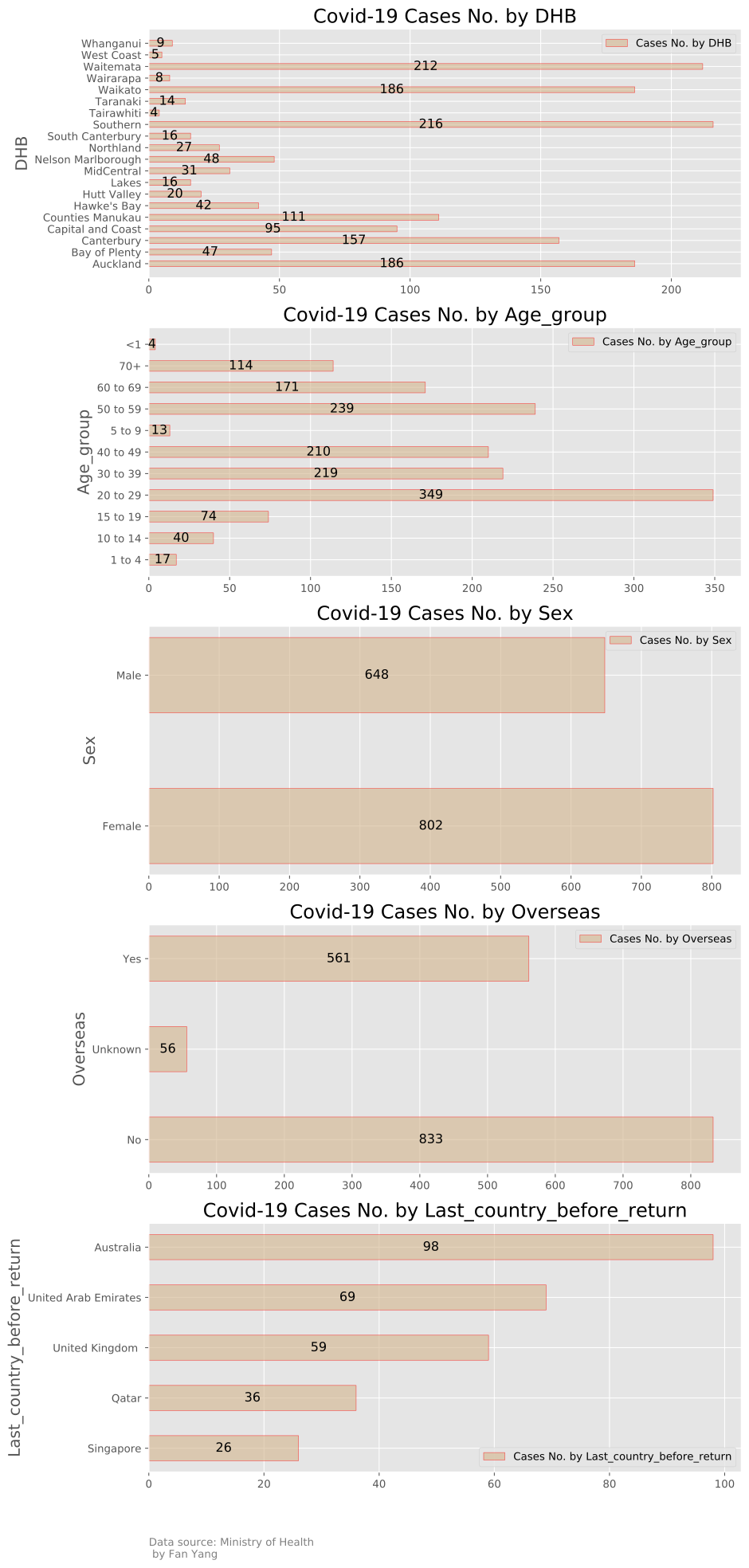
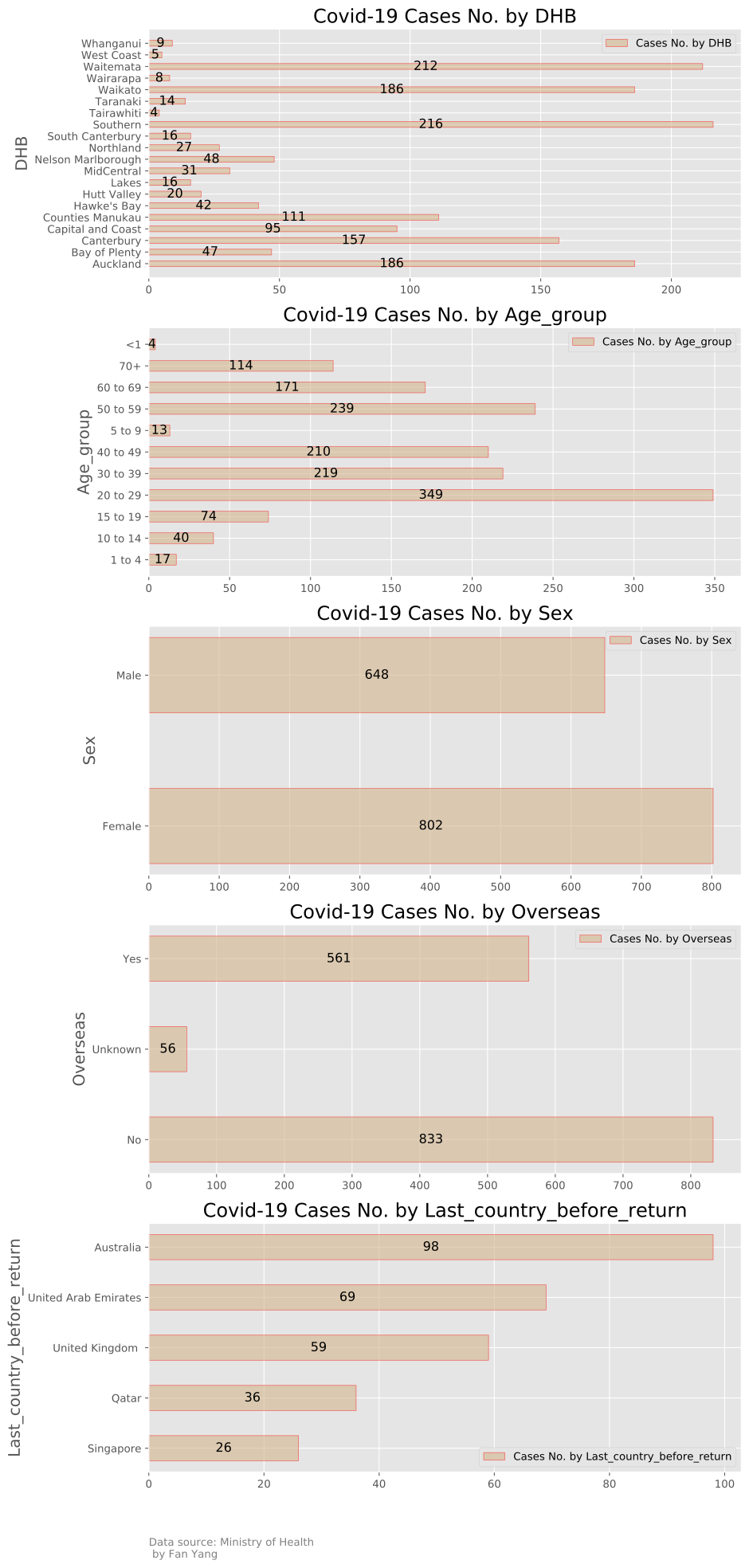
def bar_plot(AX,DF):

    AX.barh(DF.index,DF.values, height = 0.5, facecolor='tan',edgecolor='r',alpha=0.6,label = 'Cases No. by {}'.format(DF.index.name))
    AX.legend()

    AX.set_title('Covid-19 Cases No. by {}'.format(DF.index.name), fontsize = 18)
    AX.set_ylabel(DF.index.name, fontsize = 15)


    ylist = range(len(DF.values))
    for x,y in zip(DF.values, ylist):
        AX.text(x/2,y,'{}'.format(x),ha='center', va='center', fontsize = 12, color = 'black')
    if i ==4:
        ax[i,0].text(0, -2, 'Data source: Ministry of Health\n by Fan Yang', ha='left', va='center', fontsize=10,color='grey')
dfList = [df_DHB, df_age, df_gender, df_info,df_city]
fig, ax = plt.subplots(5,figsize=(10,25), squeeze = False)
Plotting data into each ax
for i in range(5):
   bar_plot(ax[i,0],dfList[i])
fig
fig
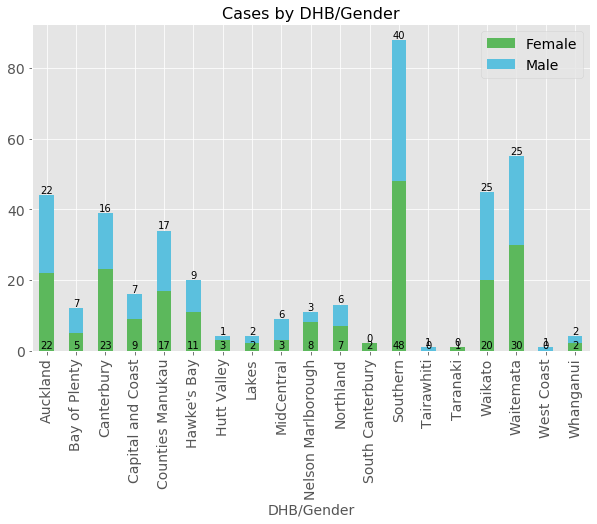
Plotting Cases by DHB/Gender
df3=df.groupby(['DHB','Sex']).count()

df3 = df3.iloc[:,1]
df3 = df3.unstack().fillna(0).astype('int32')
df3.head()
| Sex |
Female |
Male |
| DHB |
|
|
| Auckland |
22 |
22 |
| Bay of Plenty |
5 |
7 |
| Canterbury |
23 |
16 |
| Capital and Coast |
9 |
7 |
| Counties Manukau |
17 |
17 |
df3 = df3.iloc[:,:2]
#Cluster Bar Plot
xlist =list(range(0,len(df['DHB'])))

width = 0.3 #width of columns

x1 = [i-width for i in xlist]
x2 = [i+width for i in xlist]

ax = df3.plot(kind='bar',stacked=True, figsize=(10, 6), color = color_list)


ax.set_title('Cases by DHB/Gender', size = 16)
ax.set_xlabel('DHB/Gender',fontsize = 14)
ax.tick_params(labelsize=14)
ax.legend(fontsize = 14)

for x,y in zip(xlist,df3.Female):
    ax.text(x,0,r'{}'.format(y),ha='center', va='bottom', fontsize = 10)
for x,y,z in zip(xlist,df3.Male,df3.Female):
    ax.text(x,(z+y),r'{}'.format(y),ha='center', va='bottom', fontsize = 10)
Data Preparing
df5=df.groupby(['Report_Date','DHB']).count()
df5.head()
|
|
Sex |
Age_group |
Overseas |
Last_country_before_return |
| Report_Date |
DHB |
|
|
|
|
| 2020-02-26 |
Auckland |
1 |
1 |
1 |
1 |
| 2020-03-02 |
Waitemata |
1 |
1 |
1 |
1 |
| 2020-03-04 |
Counties Manukau |
1 |
1 |
1 |
0 |
| Waitemata |
1 |
1 |
1 |
1 |
| 2020-03-05 |
Counties Manukau |
1 |
1 |
1 |
1 |
dhb_sr = df5.iloc[:,1]
dhb_sr
Report_Date  DHB
2020-02-26   Auckland            1
2020-03-02   Waitemata           1
2020-03-04   Counties Manukau    1
             Waitemata           1
2020-03-05   Counties Manukau    1
                                ..
2020-04-21   Canterbury          2
             Waikato             1
2020-04-22   Canterbury          2
             Counties Manukau    1
             Hawke's Bay         1
Name: Age_group, Length: 375, dtype: int64
df5 = dhb_sr.unstack().fillna(0).astype('int32')
df5.head()
| DHB |
Auckland |
Bay of Plenty |
Canterbury |
Capital and Coast |
Counties Manukau |
Hawke's Bay |
Hutt Valley |
Lakes |
MidCentral |
Nelson Marlborough |
Northland |
South Canterbury |
Southern |
Tairawhiti |
Taranaki |
Waikato |
Wairarapa |
Waitemata |
West Coast |
Whanganui |
| Report_Date |
|
|
|
|
|
|
|
|
|
|
|
|
|
|
|
|
|
|
|
|
| 2020-02-26 |
1 |
0 |
0 |
0 |
0 |
0 |
0 |
0 |
0 |
0 |
0 |
0 |
0 |
0 |
0 |
0 |
0 |
0 |
0 |
0 |
| 2020-03-02 |
0 |
0 |
0 |
0 |
0 |
0 |
0 |
0 |
0 |
0 |
0 |
0 |
0 |
0 |
0 |
0 |
0 |
1 |
0 |
0 |
| 2020-03-04 |
0 |
0 |
0 |
0 |
1 |
0 |
0 |
0 |
0 |
0 |
0 |
0 |
0 |
0 |
0 |
0 |
0 |
1 |
0 |
0 |
| 2020-03-05 |
0 |
0 |
0 |
0 |
1 |
0 |
0 |
0 |
0 |
0 |
0 |
0 |
0 |
0 |
0 |
0 |
0 |
1 |
0 |
0 |
| 2020-03-06 |
0 |
0 |
0 |
0 |
1 |
0 |
0 |
0 |
0 |
0 |
0 |
0 |
0 |
0 |
0 |
0 |
0 |
0 |
0 |
0 |
# to calculated to accumulated case no to the specific day
df6 = df5
for i in range(len(df6.index)):
    if i == 0:
        pass
    else:
        df6.iloc[i,:] = df6.iloc[i,:] + df6.iloc[i-1,:]
df6.tail()
| DHB |
Auckland |
Bay of Plenty |
Canterbury |
Capital and Coast |
Counties Manukau |
Hawke's Bay |
Hutt Valley |
Lakes |
MidCentral |
Nelson Marlborough |
Northland |
South Canterbury |
Southern |
Tairawhiti |
Taranaki |
Waikato |
Wairarapa |
Waitemata |
West Coast |
Whanganui |
| Report_Date |
|
|
|
|
|
|
|
|
|
|
|
|
|
|
|
|
|
|
|
|
| 2020-04-18 |
185 |
45 |
150 |
93 |
110 |
41 |
20 |
16 |
31 |
48 |
27 |
15 |
216 |
4 |
14 |
184 |
8 |
211 |
5 |
8 |
| 2020-04-19 |
185 |
47 |
153 |
93 |
110 |
41 |
20 |
16 |
31 |
48 |
27 |
16 |
216 |
4 |
14 |
185 |
8 |
212 |
5 |
9 |
| 2020-04-20 |
185 |
47 |
154 |
95 |
110 |
41 |
20 |
16 |
31 |
48 |
27 |
16 |
216 |
4 |
14 |
185 |
8 |
212 |
5 |
9 |
| 2020-04-21 |
186 |
47 |
156 |
95 |
110 |
41 |
20 |
16 |
31 |
48 |
27 |
16 |
216 |
4 |
14 |
186 |
8 |
212 |
5 |
9 |
| 2020-04-22 |
186 |
47 |
158 |
95 |
111 |
42 |
20 |
16 |
31 |
48 |
27 |
16 |
216 |
4 |
14 |
186 |
8 |
212 |
5 |
9 |
# to calculated to accumulated case no to the specific day by applying the pandas function
df66 = df5.cumsum()
df66.tail()
| DHB |
Auckland |
Bay of Plenty |
Canterbury |
Capital and Coast |
Counties Manukau |
Hawke's Bay |
Hutt Valley |
Lakes |
MidCentral |
Nelson Marlborough |
Northland |
South Canterbury |
Southern |
Tairawhiti |
Taranaki |
Waikato |
Wairarapa |
Waitemata |
West Coast |
Whanganui |
| Report_Date |
|
|
|
|
|
|
|
|
|
|
|
|
|
|
|
|
|
|
|
|
| 2020-04-18 |
185 |
45 |
150 |
93 |
110 |
41 |
20 |
16 |
31 |
48 |
27 |
15 |
216 |
4 |
14 |
184 |
8 |
211 |
5 |
8 |
| 2020-04-19 |
185 |
47 |
153 |
93 |
110 |
41 |
20 |
16 |
31 |
48 |
27 |
16 |
216 |
4 |
14 |
185 |
8 |
212 |
5 |
9 |
| 2020-04-20 |
185 |
47 |
154 |
95 |
110 |
41 |
20 |
16 |
31 |
48 |
27 |
16 |
216 |
4 |
14 |
185 |
8 |
212 |
5 |
9 |
| 2020-04-21 |
186 |
47 |
156 |
95 |
110 |
41 |
20 |
16 |
31 |
48 |
27 |
16 |
216 |
4 |
14 |
186 |
8 |
212 |
5 |
9 |
| 2020-04-22 |
186 |
47 |
158 |
95 |
111 |
42 |
20 |
16 |
31 |
48 |
27 |
16 |
216 |
4 |
14 |
186 |
8 |
212 |
5 |
9 |
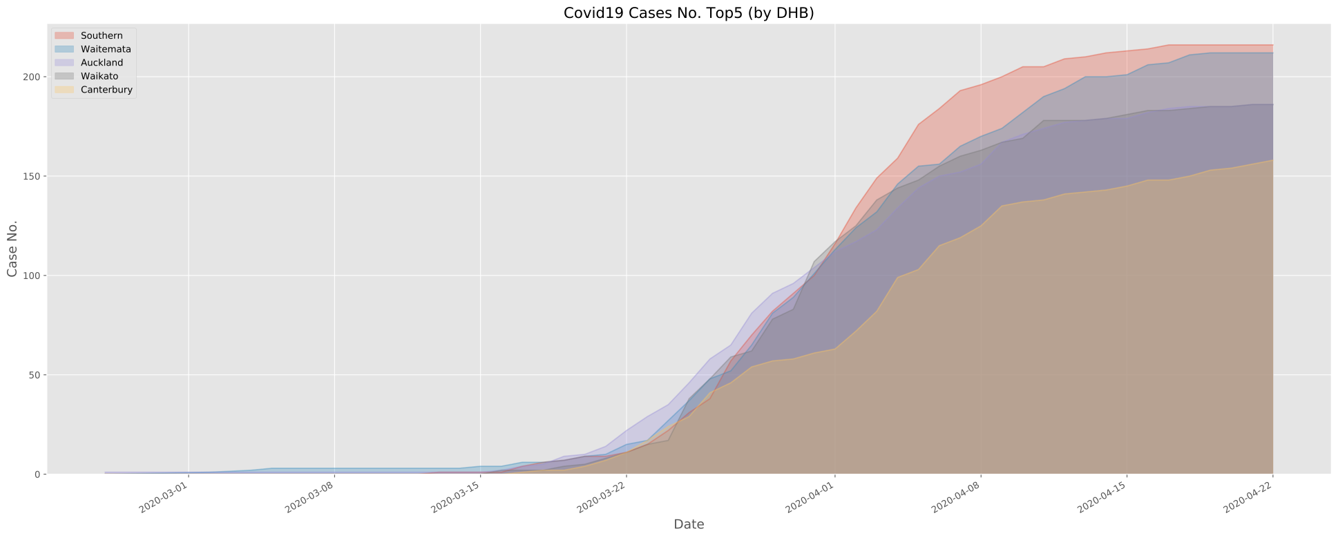
Picking up the cities with top 5 confirmed cases No.
DHBlist = df5.sum().sort_values(ascending = False) # descending rank in cases No.
DHBlist = DHBlist.head(5).index
DHBlist = DHBlist.tolist()
DHBlist
['Southern', 'Waitemata', 'Auckland', 'Waikato', 'Canterbury']
Area plot
pd.plotting.register_matplotlib_converters()
df_top5.plot(kind='area', alpha = 0.3,
             stacked = False,
             figsize=(25, 10), # pass a tuple (x, y) size
             )

plt.title('Covid19 Cases No. Top5 (by DHB)', size = 16)
plt.xlabel('Date',fontsize = 14)
plt.ylabel('Case No.',fontsize = 14)

plt.legend()
<matplotlib.legend.Legend at 0x22525b8bbc8>
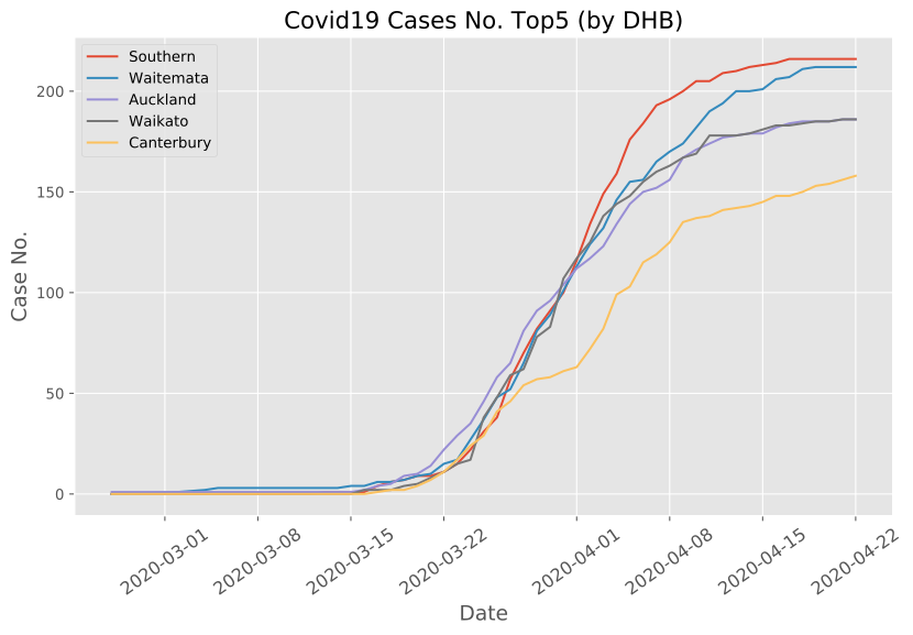
Line plot
fig, ax = plt.subplots(figsize = (10,6))

for i in range(len(df_top5.columns)):
    ax.plot(df_top5.index,df_top5.iloc[:,i].values,label = df_top5.columns[i])

ax.set_title('Covid19 Cases No. Top5 (by DHB)', size = 16)
ax.set_xlabel('Date',fontsize = 14)
ax.set_ylabel('Case No.',fontsize = 14)


ax.xaxis.set_tick_params(rotation = 35, labelsize = 12)


ax.legend()
Reference
https://www.health.govt.nz/our-work/diseases-and-conditions/covid-19-novel-coronavirus/covid-19-current-situation/covid-19-current-cases/covid-19-current-cases-details