Import the packages and files
%matplotlib inline #static images of your plot embedded in the notebook
Import the related package
import geopandas as gpd
import numpy as np
import matplotlib.pyplot  as plt
import pandas as pd
from shapely.geometry import Point
Read the city point shape file and city boundary polyline file
states = gpd.read_file('D:\ARCGIS\Covid-19 Cases in New Zealand\output\DHI_POINTS.shp')
cities = gpd.read_file('D:\ARCGIS\Covid-19 Cases in New Zealand\output\Export_Output_3.shp')
Data Wrangling
states = states.iloc[:,[3,4,-1]]
states.head(2)
| DHB2015_Na | Shape_Leng | geometry | |
|---|---|---|---|
| 0 | Northland | 1.651929e+06 | POINT (173.82591 -35.48993) |
| 1 | Waitemata | 9.273920e+05 | POINT (174.54665 -36.56396) |
states.index
RangeIndex(start=0, stop=20, step=1)
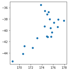
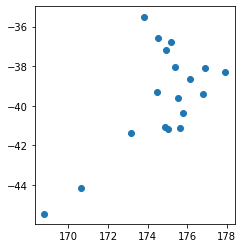
states.plot()
<matplotlib.axes._subplots.AxesSubplot at 0x1c22a6044e0>
cities
| OBJECTID | DHB2015_Co | DHB2015_Na | Shape_Leng | Shape_Le_1 | Shape_Area | geometry | |
|---|---|---|---|---|---|---|---|
| 0 | 1 | 01 | Northland | 1.651929e+06 | 16.524423 | 1.320491 | MULTIPOLYGON (((174.23335 -36.19077, 174.23809... |
| 1 | 2 | 02 | Waitemata | 9.273920e+05 | 9.301324 | 0.295480 | MULTIPOLYGON (((174.77898 -36.82617, 174.77303... |
| 2 | 3 | 03 | Auckland | 7.781903e+05 | 7.848241 | 0.063644 | MULTIPOLYGON (((175.16845 -36.90380, 175.15541... |
| 3 | 4 | 04 | Counties Manukau | 6.642233e+05 | 6.732029 | 0.303391 | POLYGON ((174.72654 -37.15219, 174.74646 -37.1... |
| 4 | 5 | 05 | Waikato | 1.498296e+06 | 15.120324 | 2.201743 | MULTIPOLYGON (((175.95463 -37.04760, 175.93959... |
| 5 | 6 | 06 | Lakes | 6.236689e+05 | 6.356743 | 0.990685 | POLYGON ((176.60295 -38.01159, 176.57811 -38.4... |
| 6 | 7 | 07 | Bay of Plenty | 9.468737e+05 | 9.636408 | 1.014598 | MULTIPOLYGON (((176.43654 -37.62005, 176.40701... |
| 7 | 8 | 08 | Tairawhiti | 6.895486e+05 | 7.001250 | 0.860188 | MULTIPOLYGON (((178.35631 -38.17577, 178.36485... |
| 8 | 9 | 09 | Taranaki | 5.657958e+05 | 5.886723 | 0.830015 | POLYGON ((174.98759 -39.66387, 174.78429 -39.8... |
| 9 | 10 | 10 | Hawke's Bay | 9.454397e+05 | 9.687377 | 1.335790 | MULTIPOLYGON (((177.87052 -39.27876, 177.86687... |
| 10 | 11 | 11 | Whanganui | 6.694279e+05 | 6.927098 | 1.003196 | POLYGON ((176.29008 -39.24717, 176.26502 -39.3... |
| 11 | 12 | 12 | MidCentral | 6.167762e+05 | 6.345139 | 0.937664 | POLYGON ((176.49213 -40.53208, 176.26669 -40.7... |
| 12 | 13 | 13 | Hutt Valley | 2.106983e+05 | 2.184028 | 0.098310 | MULTIPOLYGON (((174.86764 -41.25918, 174.86522... |
| 13 | 14 | 14 | Capital and Coast | 2.923868e+05 | 3.012962 | 0.080068 | MULTIPOLYGON (((174.78879 -41.09057, 174.77354... |
| 14 | 15 | 15 | Wairarapa | 4.554528e+05 | 4.751018 | 0.636207 | POLYGON ((176.27048 -40.74387, 176.26669 -40.7... |
| 15 | 16 | 16 | Nelson Marlborough | 1.188104e+06 | 12.372261 | 2.986687 | POLYGON ((173.36103 -40.80538, 173.20652 -41.2... |
| 16 | 17 | 17 | West Coast | 1.602904e+06 | 17.070329 | 2.569502 | POLYGON ((172.31080 -41.01154, 172.32531 -41.0... |
| 17 | 19 | 19 | South Canterbury | 5.492453e+05 | 5.835052 | 1.547516 | POLYGON ((170.61509 -43.43343, 170.59805 -43.4... |
| 18 | 20 | 22 | Southern | 2.725169e+06 | 30.268153 | 7.932661 | MULTIPOLYGON (((167.39897 -47.26532, 167.39639... |
cities.drop(axis=0,  columns=['DHB2015_Co'],inplace=True)
cities.head(2)
| OBJECTID | DHB2015_Na | Shape_Leng | Shape_Le_1 | Shape_Area | geometry | |
|---|---|---|---|---|---|---|
| 0 | 1 | Northland | 1.651929e+06 | 16.524423 | 1.320491 | MULTIPOLYGON (((174.23335 -36.19077, 174.23809... |
| 1 | 2 | Waitemata | 9.273920e+05 | 9.301324 | 0.295480 | MULTIPOLYGON (((174.77898 -36.82617, 174.77303... |
cities.index
RangeIndex(start=0, stop=19, step=1)
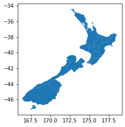
cities.plot()
<matplotlib.axes._subplots.AxesSubplot at 0x1c22a63b5f8>
Spatial Join
Column join in Pandas-- take dataset A+ B based on a common column
Spatial Join -take dataset A+B = Dataset AB,based on space/geographic relationship
same as the spatial join in ArcGis, but it much more convient to use than Arcpy
Check the coordinate systems of the to two taget file, if they are not in the same coordinate system, then project them into the same coordinate system
print(states.crs, cities.crs)
epsg:4326 epsg:4326
states.to_crs(cities.crs, inplace =True)
len(states)
20
states_with_cities = gpd.sjoin(states, cities, how = 'inner', op = 'within')
states_with_cities.head(2)
| DHB2015_Na_left | Shape_Leng_left | geometry | index_right | OBJECTID | DHB2015_Na_right | Shape_Leng_right | Shape_Le_1 | Shape_Area | |
|---|---|---|---|---|---|---|---|---|---|
| 0 | Northland | 1.651929e+06 | POINT (173.82591 -35.48993) | 0 | 1 | Northland | 1.651929e+06 | 16.524423 | 1.320491 |
| 1 | Waitemata | 9.273920e+05 | POINT (174.54665 -36.56396) | 1 | 2 | Waitemata | 9.273920e+05 | 9.301324 | 0.295480 |
states_with_cities.shape
(18, 9)
states.shape
(20, 3)
The order here is very important, similar as the join in pandas.
The geometry of the first file(cities here) is will be kept.
how:
- ‘Left’ means to keep all the information in the first file even they do not have matching state
- ‘inner’ means to drop the information in the first file if they do not have matching state
cities_with_states = gpd.sjoin(cities, states, how = 'inner', op = 'contains')
cities_with_states.head(2)
| OBJECTID | DHB2015_Na_left | Shape_Leng_left | Shape_Le_1 | Shape_Area | geometry | index_right | DHB2015_Na_right | Shape_Leng_right | |
|---|---|---|---|---|---|---|---|---|---|
| 0 | 1 | Northland | 1.651929e+06 | 16.524423 | 1.320491 | MULTIPOLYGON (((174.23335 -36.19077, 174.23809... | 0 | Northland | 1.651929e+06 |
| 1 | 2 | Waitemata | 9.273920e+05 | 9.301324 | 0.295480 | MULTIPOLYGON (((174.77898 -36.82617, 174.77303... | 1 | Waitemata | 9.273920e+05 |
cities_with_states.shape
(18, 9)
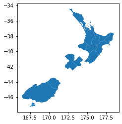
gpd.sjoin(cities, states, how = 'inner', op = 'contains').plot()
<matplotlib.axes._subplots.AxesSubplot at 0x1c22a6cdbe0>
gpd.sjoin(cities, states, how = 'left', op = 'contains').plot()
<matplotlib.axes._subplots.AxesSubplot at 0x1c22a3f0710>
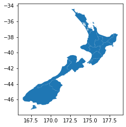
gpd.sjoin(cities, states, how = 'left', op = 'contains').shape
(19, 9)
Another way
states_with_cities = gpd.sjoin(states, cities, how = 'inner', op = 'within')
states_with_cities.head()
| DHB2015_Na_left | Shape_Leng_left | geometry | index_right | OBJECTID | DHB2015_Na_right | Shape_Leng_right | Shape_Le_1 | Shape_Area | |
|---|---|---|---|---|---|---|---|---|---|
| 0 | Northland | 1.651929e+06 | POINT (173.82591 -35.48993) | 0 | 1 | Northland | 1.651929e+06 | 16.524423 | 1.320491 |
| 1 | Waitemata | 9.273920e+05 | POINT (174.54665 -36.56396) | 1 | 2 | Waitemata | 9.273920e+05 | 9.301324 | 0.295480 |
| 2 | Auckland | 7.781903e+05 | POINT (175.15511 -36.78522) | 2 | 3 | Auckland | 7.781903e+05 | 7.848241 | 0.063644 |
| 3 | Counties Manukau | 6.642233e+05 | POINT (174.93239 -37.18770) | 3 | 4 | Counties Manukau | 6.642233e+05 | 6.732029 | 0.303391 |
| 4 | Waikato | 1.498296e+06 | POINT (175.35693 -38.04867) | 4 | 5 | Waikato | 1.498296e+06 | 15.120324 | 2.201743 |
states_with_cities.shape
(18, 9)
states_with_cities.plot()
<matplotlib.axes._subplots.AxesSubplot at 0x1c22a7317f0>
gpd.sjoin(states, cities, how = 'left', op = 'within').shape
(20, 9)
Here, the shape is different from the previous one(19,9), since the data of all the states is kept, then final joined result is same as the source data(states).
Reference
https://geopandas.org/install.html#dependencies
https://www.youtube.com/watch?v=mV8bqV2j46M&list=PLewNEVDy7gq3DjrPDxGFLbHE4G2QWe8Qh&index=12