Introduction to Matplotlib and Line Plots

Table of Contents

1. Exploring Datasets with pandas
   1.1 The Dataset: Immigration to Canada from 1980 to 2013
   1.2 pandas Basics
   1.3 pandas Intermediate: Indexing and Selection
   

2. Visualizing Data using Matplotlib
   2.1 Matplotlib: Standard Python Visualization Library
   

3. Line Plots

---

Exploring Datasets with pandas

pandas is an essential data analysis toolkit for Python. From their website:

pandas is a Python package providing fast, flexible, and expressive data structures designed to make working with “relational” or “labeled” data both easy and intuitive. It aims to be the fundamental high-level building block for doing practical, real world data analysis in Python.

The course heavily relies on pandas for data wrangling, analysis, and visualization. We encourage you to spend some time and familizare yourself with the pandas API Reference: http://pandas.pydata.org/pandas-docs/stable/api.html.

The Dataset: Immigration to Canada from 1980 to 2013

pandas Basics

The first thing we’ll do is import two key data analysis modules: pandas and Numpy.

import numpy as np  # useful for many scientific computing in Python
import pandas as pd # primary data structure library

Now we are ready to read in our data.

df_can = pd.read_excel('Canada.xlsx',
                       sheet_name='Canada by Citizenship',
                       skiprows=range(20),
                       skipfooter=2)

print ('Data read into a pandas dataframe!')

Data read into a pandas dataframe!

Let’s view the top 5 rows of the dataset using the head() function.

df_can.head()
# tip: You can specify the number of rows you'd like to see as follows: df_can.head(10)

	Type	Coverage	OdName	AREA	AreaName	REG	RegName	DEV	DevName	1980	...	2004	2005	2006	2007	2008	2009	2010	2011	2012	2013
0	Immigrants	Foreigners	Afghanistan	935	Asia	5501	Southern Asia	902	Developing regions	16	...	2978	3436	3009	2652	2111	1746	1758	2203	2635	2004
1	Immigrants	Foreigners	Albania	908	Europe	925	Southern Europe	901	Developed regions	1	...	1450	1223	856	702	560	716	561	539	620	603
2	Immigrants	Foreigners	Algeria	903	Africa	912	Northern Africa	902	Developing regions	80	...	3616	3626	4807	3623	4005	5393	4752	4325	3774	4331
3	Immigrants	Foreigners	American Samoa	909	Oceania	957	Polynesia	902	Developing regions	0	...	0	0	1	0	0	0	0	0	0	0
4	Immigrants	Foreigners	Andorra	908	Europe	925	Southern Europe	901	Developed regions	0	...	0	0	1	1	0	0	0	0	1	1

5 rows × 43 columns

We can also veiw the bottom 5 rows of the dataset using the tail() function.

df_can.tail()

	Type	Coverage	OdName	AREA	AreaName	REG	RegName	DEV	DevName	1980	...	2004	2005	2006	2007	2008	2009	2010	2011	2012	2013
190	Immigrants	Foreigners	Viet Nam	935	Asia	920	South-Eastern Asia	902	Developing regions	1191	...	1816	1852	3153	2574	1784	2171	1942	1723	1731	2112
191	Immigrants	Foreigners	Western Sahara	903	Africa	912	Northern Africa	902	Developing regions	0	...	0	0	1	0	0	0	0	0	0	0
192	Immigrants	Foreigners	Yemen	935	Asia	922	Western Asia	902	Developing regions	1	...	124	161	140	122	133	128	211	160	174	217
193	Immigrants	Foreigners	Zambia	903	Africa	910	Eastern Africa	902	Developing regions	11	...	56	91	77	71	64	60	102	69	46	59
194	Immigrants	Foreigners	Zimbabwe	903	Africa	910	Eastern Africa	902	Developing regions	72	...	1450	615	454	663	611	508	494	434	437	407

5 rows × 43 columns

When analyzing a dataset, it’s always a good idea to start by getting basic information about your dataframe. We can do this by using the info() method.

df_can.info()

<class 'pandas.core.frame.DataFrame'>
RangeIndex: 195 entries, 0 to 194
Data columns (total 43 columns):
Type        195 non-null object
Coverage    195 non-null object
OdName      195 non-null object
AREA        195 non-null int64
AreaName    195 non-null object
REG         195 non-null int64
RegName     195 non-null object
DEV         195 non-null int64
DevName     195 non-null object
1980        195 non-null int64
1981        195 non-null int64
1982        195 non-null int64
1983        195 non-null int64
1984        195 non-null int64
1985        195 non-null int64
1986        195 non-null int64
1987        195 non-null int64
1988        195 non-null int64
1989        195 non-null int64
1990        195 non-null int64
1991        195 non-null int64
1992        195 non-null int64
1993        195 non-null int64
1994        195 non-null int64
1995        195 non-null int64
1996        195 non-null int64
1997        195 non-null int64
1998        195 non-null int64
1999        195 non-null int64
2000        195 non-null int64
2001        195 non-null int64
2002        195 non-null int64
2003        195 non-null int64
2004        195 non-null int64
2005        195 non-null int64
2006        195 non-null int64
2007        195 non-null int64
2008        195 non-null int64
2009        195 non-null int64
2010        195 non-null int64
2011        195 non-null int64
2012        195 non-null int64
2013        195 non-null int64
dtypes: int64(37), object(6)
memory usage: 65.6+ KB

To get the list of column headers we can call upon the dataframe’s .columns parameter.

df_can.columns.values

array(['Type', 'Coverage', 'OdName', 'AREA', 'AreaName', 'REG', 'RegName',
       'DEV', 'DevName', 1980, 1981, 1982, 1983, 1984, 1985, 1986, 1987,
       1988, 1989, 1990, 1991, 1992, 1993, 1994, 1995, 1996, 1997, 1998,
       1999, 2000, 2001, 2002, 2003, 2004, 2005, 2006, 2007, 2008, 2009,
       2010, 2011, 2012, 2013], dtype=object)

Similarly, to get the list of indicies we use the .index parameter.

df_can.index.values

array([  0,   1,   2,   3,   4,   5,   6,   7,   8,   9,  10,  11,  12,
        13,  14,  15,  16,  17,  18,  19,  20,  21,  22,  23,  24,  25,
        26,  27,  28,  29,  30,  31,  32,  33,  34,  35,  36,  37,  38,
        39,  40,  41,  42,  43,  44,  45,  46,  47,  48,  49,  50,  51,
        52,  53,  54,  55,  56,  57,  58,  59,  60,  61,  62,  63,  64,
        65,  66,  67,  68,  69,  70,  71,  72,  73,  74,  75,  76,  77,
        78,  79,  80,  81,  82,  83,  84,  85,  86,  87,  88,  89,  90,
        91,  92,  93,  94,  95,  96,  97,  98,  99, 100, 101, 102, 103,
       104, 105, 106, 107, 108, 109, 110, 111, 112, 113, 114, 115, 116,
       117, 118, 119, 120, 121, 122, 123, 124, 125, 126, 127, 128, 129,
       130, 131, 132, 133, 134, 135, 136, 137, 138, 139, 140, 141, 142,
       143, 144, 145, 146, 147, 148, 149, 150, 151, 152, 153, 154, 155,
       156, 157, 158, 159, 160, 161, 162, 163, 164, 165, 166, 167, 168,
       169, 170, 171, 172, 173, 174, 175, 176, 177, 178, 179, 180, 181,
       182, 183, 184, 185, 186, 187, 188, 189, 190, 191, 192, 193, 194],
      dtype=int64)

Note: The default type of index and columns is NOT list.

print(type(df_can.columns))
print(type(df_can.index))

<class 'pandas.core.indexes.base.Index'>
<class 'pandas.core.indexes.range.RangeIndex'>

To get the index and columns as lists, we can use the tolist() method.

df_can.columns.tolist()
df_can.index.tolist()

print (type(df_can.columns.tolist()))
print (type(df_can.index.tolist()))

<class 'list'>
<class 'list'>

To view the dimensions of the dataframe, we use the .shape parameter.

# size of dataframe (rows, columns)
df_can.shape    

(195, 43)

Note: The main types stored in pandas objects are float, int, bool, datetime64[ns] and datetime64[ns, tz] (in >= 0.17.0), timedelta[ns], category (in >= 0.15.0), and object (string). In addition these dtypes have item sizes, e.g. int64 and int32.

Let’s clean the data set to remove a few unnecessary columns. We can use pandas drop() method as follows:

# in pandas axis=0 represents rows (default) and axis=1 represents columns.
df_can.drop(['AREA','REG','DEV','Type','Coverage'], axis=1, inplace=True)
df_can.head(2)

	OdName	AreaName	RegName	DevName	1980	1981	1982	1983	1984	1985	...	2004	2005	2006	2007	2008	2009	2010	2011	2012	2013
0	Afghanistan	Asia	Southern Asia	Developing regions	16	39	39	47	71	340	...	2978	3436	3009	2652	2111	1746	1758	2203	2635	2004
1	Albania	Europe	Southern Europe	Developed regions	1	0	0	0	0	0	...	1450	1223	856	702	560	716	561	539	620	603

2 rows × 38 columns

Let’s rename the columns so that they make sense. We can use rename() method by passing in a dictionary of old and new names as follows:

df_can.rename(columns={'OdName':'Country', 'AreaName':'Continent', 'RegName':'Region'}, inplace=True)
df_can.columns

Index([  'Country', 'Continent',    'Region',   'DevName',        1980,
              1981,        1982,        1983,        1984,        1985,
              1986,        1987,        1988,        1989,        1990,
              1991,        1992,        1993,        1994,        1995,
              1996,        1997,        1998,        1999,        2000,
              2001,        2002,        2003,        2004,        2005,
              2006,        2007,        2008,        2009,        2010,
              2011,        2012,        2013],
      dtype='object')

We will also add a ‘Total’ column that sums up the total immigrants by country over the entire period 1980 - 2013, as follows:

df_can['Total'] = df_can.sum(axis=1)

We can check to see how many null objects we have in the dataset as follows:

df_can.isnull().sum()

Country      0
Continent    0
Region       0
DevName      0
1980         0
1981         0
1982         0
1983         0
1984         0
1985         0
1986         0
1987         0
1988         0
1989         0
1990         0
1991         0
1992         0
1993         0
1994         0
1995         0
1996         0
1997         0
1998         0
1999         0
2000         0
2001         0
2002         0
2003         0
2004         0
2005         0
2006         0
2007         0
2008         0
2009         0
2010         0
2011         0
2012         0
2013         0
Total        0
dtype: int64

Finally, let’s view a quick summary of each column in our dataframe using the describe() method.

df_can.describe()

	1980	1981	1982	1983	1984	1985	1986	1987	1988	1989	...	2005	2006	2007	2008	2009	2010	2011	2012	2013	Total
count	195.000000	195.000000	195.000000	195.000000	195.000000	195.000000	195.000000	195.000000	195.000000	195.000000	...	195.000000	195.000000	195.000000	195.000000	195.000000	195.000000	195.000000	195.000000	195.000000	195.000000
mean	508.394872	566.989744	534.723077	387.435897	376.497436	358.861538	441.271795	691.133333	714.389744	843.241026	...	1320.292308	1266.958974	1191.820513	1246.394872	1275.733333	1420.287179	1262.533333	1313.958974	1320.702564	32867.451282
std	1949.588546	2152.643752	1866.997511	1204.333597	1198.246371	1079.309600	1225.576630	2109.205607	2443.606788	2555.048874	...	4425.957828	3926.717747	3443.542409	3694.573544	3829.630424	4462.946328	4030.084313	4247.555161	4237.951988	91785.498686
min	0.000000	0.000000	0.000000	0.000000	0.000000	0.000000	0.000000	0.000000	0.000000	0.000000	...	0.000000	0.000000	0.000000	0.000000	0.000000	0.000000	0.000000	0.000000	0.000000	1.000000
25%	0.000000	0.000000	0.000000	0.000000	0.000000	0.000000	0.500000	0.500000	1.000000	1.000000	...	28.500000	25.000000	31.000000	31.000000	36.000000	40.500000	37.500000	42.500000	45.000000	952.000000
50%	13.000000	10.000000	11.000000	12.000000	13.000000	17.000000	18.000000	26.000000	34.000000	44.000000	...	210.000000	218.000000	198.000000	205.000000	214.000000	211.000000	179.000000	233.000000	213.000000	5018.000000
75%	251.500000	295.500000	275.000000	173.000000	181.000000	197.000000	254.000000	434.000000	409.000000	508.500000	...	832.000000	842.000000	899.000000	934.500000	888.000000	932.000000	772.000000	783.000000	796.000000	22239.500000
max	22045.000000	24796.000000	20620.000000	10015.000000	10170.000000	9564.000000	9470.000000	21337.000000	27359.000000	23795.000000	...	42584.000000	33848.000000	28742.000000	30037.000000	29622.000000	38617.000000	36765.000000	34315.000000	34129.000000	691904.000000

8 rows × 35 columns

---

pandas Intermediate: Indexing and Selection (slicing)

Select Column

There are two ways to filter on a column name:

Method 1: Quick and easy, but only works if the column name does NOT have spaces or special characters.

    df.column_name
        (returns series)

Method 2: More robust, and can filter on multiple columns.

    df['column']  
        (returns series)

    df[['column 1', 'column 2']]
        (returns dataframe)

---

Example: Let’s try filtering on the list of countries (‘Country’).

df_can.Country  # returns a series

0         Afghanistan
1             Albania
2             Algeria
3      American Samoa
4             Andorra
            ...      
190          Viet Nam
191    Western Sahara
192             Yemen
193            Zambia
194          Zimbabwe
Name: Country, Length: 195, dtype: object

Let’s try filtering on the list of countries (‘OdName’) and the data for years: 1980 - 1985.

df_can[['Country', 1980, 1981, 1982, 1983, 1984, 1985]] # returns a dataframe
# notice that 'Country' is string, and the years are integers.
# for the sake of consistency, we will convert all column names to string later on.

	Country	1980	1981	1982	1983	1984	1985
0	Afghanistan	16	39	39	47	71	340
1	Albania	1	0	0	0	0	0
2	Algeria	80	67	71	69	63	44
3	American Samoa	0	1	0	0	0	0
4	Andorra	0	0	0	0	0	0
...	...	...	...	...	...	...	...
190	Viet Nam	1191	1829	2162	3404	7583	5907
191	Western Sahara	0	0	0	0	0	0
192	Yemen	1	2	1	6	0	18
193	Zambia	11	17	11	7	16	9
194	Zimbabwe	72	114	102	44	32	29

195 rows × 7 columns

df_can.head()

	Country	Continent	Region	DevName	1980	1981	1982	1983	1984	1985	...	2005	2006	2007	2008	2009	2010	2011	2012	2013	Total
0	Afghanistan	Asia	Southern Asia	Developing regions	16	39	39	47	71	340	...	3436	3009	2652	2111	1746	1758	2203	2635	2004	58639
1	Albania	Europe	Southern Europe	Developed regions	1	0	0	0	0	0	...	1223	856	702	560	716	561	539	620	603	15699
2	Algeria	Africa	Northern Africa	Developing regions	80	67	71	69	63	44	...	3626	4807	3623	4005	5393	4752	4325	3774	4331	69439
3	American Samoa	Oceania	Polynesia	Developing regions	0	1	0	0	0	0	...	0	1	0	0	0	0	0	0	0	6
4	Andorra	Europe	Southern Europe	Developed regions	0	0	0	0	0	0	...	0	1	1	0	0	0	0	1	1	15

5 rows × 39 columns

Select Row

There are main 3 ways to select rows:

    df.loc[label]        
        #filters by the labels of the index/column
    df.iloc[index]       
        #filters by the positions of the index/column

Before we proceed, notice that the defaul index of the dataset is a numeric range from 0 to 194. This makes it very difficult to do a query by a specific country. For example to search for data on Japan, we need to know the corressponding index value.

This can be fixed very easily by setting the ‘Country’ column as the index using set_index() method.

df_can.set_index('Country', inplace=True)
# tip: The opposite of set is reset. So to reset the index, we can use df_can.reset_index()

df_can.head(3)

	Continent	Region	DevName	1980	1981	1982	1983	1984	1985	1986	...	2005	2006	2007	2008	2009	2010	2011	2012	2013	Total
Country
Afghanistan	Asia	Southern Asia	Developing regions	16	39	39	47	71	340	496	...	3436	3009	2652	2111	1746	1758	2203	2635	2004	58639
Albania	Europe	Southern Europe	Developed regions	1	0	0	0	0	0	1	...	1223	856	702	560	716	561	539	620	603	15699
Algeria	Africa	Northern Africa	Developing regions	80	67	71	69	63	44	69	...	3626	4807	3623	4005	5393	4752	4325	3774	4331	69439

3 rows × 38 columns

# optional: to remove the name of the index
df_can.index.name = None

Example: Let’s view the number of immigrants from Japan (row 87) for the following scenarios:
1. The full row data (all columns)
2. For year 2013
3. For years 1980 to 1985

# 1. the full row data (all columns)
print(df_can.loc['Japan'])

# alternate methods
print(df_can.iloc[87])
print(df_can[df_can.index == 'Japan'].T.squeeze())

Continent                 Asia
Region            Eastern Asia
DevName      Developed regions
1980                       701
1981                       756
1982                       598
1983                       309
1984                       246
1985                       198
1986                       248
1987                       422
1988                       324
1989                       494
1990                       379
1991                       506
1992                       605
1993                       907
1994                       956
1995                       826
1996                       994
1997                       924
1998                       897
1999                      1083
2000                      1010
2001                      1092
2002                       806
2003                       817
2004                       973
2005                      1067
2006                      1212
2007                      1250
2008                      1284
2009                      1194
2010                      1168
2011                      1265
2012                      1214
2013                       982
Total                    27707
Name: Japan, dtype: object
Continent                 Asia
Region            Eastern Asia
DevName      Developed regions
1980                       701
1981                       756
1982                       598
1983                       309
1984                       246
1985                       198
1986                       248
1987                       422
1988                       324
1989                       494
1990                       379
1991                       506
1992                       605
1993                       907
1994                       956
1995                       826
1996                       994
1997                       924
1998                       897
1999                      1083
2000                      1010
2001                      1092
2002                       806
2003                       817
2004                       973
2005                      1067
2006                      1212
2007                      1250
2008                      1284
2009                      1194
2010                      1168
2011                      1265
2012                      1214
2013                       982
Total                    27707
Name: Japan, dtype: object
Continent                 Asia
Region            Eastern Asia
DevName      Developed regions
1980                       701
1981                       756
1982                       598
1983                       309
1984                       246
1985                       198
1986                       248
1987                       422
1988                       324
1989                       494
1990                       379
1991                       506
1992                       605
1993                       907
1994                       956
1995                       826
1996                       994
1997                       924
1998                       897
1999                      1083
2000                      1010
2001                      1092
2002                       806
2003                       817
2004                       973
2005                      1067
2006                      1212
2007                      1250
2008                      1284
2009                      1194
2010                      1168
2011                      1265
2012                      1214
2013                       982
Total                    27707
Name: Japan, dtype: object

# 2. for year 2013
print(df_can.loc['Japan', 2013])

# alternate method
print(df_can.iloc[87, 36]) # year 2013 is the last column, with a positional index of 36

982
982

# 3. for years 1980 to 1985
print(df_can.loc['Japan', [1980, 1981, 1982, 1983, 1984, 1984]])
print(df_can.iloc[87, [3, 4, 5, 6, 7, 8]])

1980    701
1981    756
1982    598
1983    309
1984    246
1984    246
Name: Japan, dtype: object
1980    701
1981    756
1982    598
1983    309
1984    246
1985    198
Name: Japan, dtype: object

Column names that are integers (such as the years) might introduce some confusion. For example, when we are referencing the year 2013, one might confuse that when the 2013th positional index.

To avoid this ambuigity, let’s convert the column names into strings: ‘1980’ to ‘2013’.

df_can.columns = list(map(str, df_can.columns))
# [print (type(x)) for x in df_can.columns.values] #<-- uncomment to check type of column headers

Since we converted the years to string, let’s declare a variable that will allow us to easily call upon the full range of years:

# useful for plotting later on
years = list(map(str, range(1980, 2014)))
years

['1980',
 '1981',
 '1982',
 '1983',
 '1984',
 '1985',
 '1986',
 '1987',
 '1988',
 '1989',
 '1990',
 '1991',
 '1992',
 '1993',
 '1994',
 '1995',
 '1996',
 '1997',
 '1998',
 '1999',
 '2000',
 '2001',
 '2002',
 '2003',
 '2004',
 '2005',
 '2006',
 '2007',
 '2008',
 '2009',
 '2010',
 '2011',
 '2012',
 '2013']

Filtering based on a criteria

To filter the dataframe based on a condition, we simply pass the condition as a boolean vector.

For example, Let’s filter the dataframe to show the data on Asian countries (AreaName = Asia).

# 1. create the condition boolean series
condition = df_can['Continent'] == 'Asia'
print(condition)

Afghanistan        True
Albania           False
Algeria           False
American Samoa    False
Andorra           False
                  ...  
Viet Nam           True
Western Sahara    False
Yemen              True
Zambia            False
Zimbabwe          False
Name: Continent, Length: 195, dtype: bool

# 2. pass this condition into the dataFrame
df_can[condition]

	Continent	Region	DevName	1980	1981	1982	1983	1984	1985	1986	...	2005	2006	2007	2008	2009	2010	2011	2012	2013	Total
Afghanistan	Asia	Southern Asia	Developing regions	16	39	39	47	71	340	496	...	3436	3009	2652	2111	1746	1758	2203	2635	2004	58639
Armenia	Asia	Western Asia	Developing regions	0	0	0	0	0	0	0	...	224	218	198	205	267	252	236	258	207	3310
Azerbaijan	Asia	Western Asia	Developing regions	0	0	0	0	0	0	0	...	359	236	203	125	165	209	138	161	57	2649
Bahrain	Asia	Western Asia	Developing regions	0	2	1	1	1	3	0	...	12	12	22	9	35	28	21	39	32	475
Bangladesh	Asia	Southern Asia	Developing regions	83	84	86	81	98	92	486	...	4171	4014	2897	2939	2104	4721	2694	2640	3789	65568
Bhutan	Asia	Southern Asia	Developing regions	0	0	0	0	1	0	0	...	5	10	7	36	865	1464	1879	1075	487	5876
Brunei Darussalam	Asia	South-Eastern Asia	Developing regions	79	6	8	2	2	4	12	...	4	5	11	10	5	12	6	3	6	600
Cambodia	Asia	South-Eastern Asia	Developing regions	12	19	26	33	10	7	8	...	370	529	460	354	203	200	196	233	288	6538
China	Asia	Eastern Asia	Developing regions	5123	6682	3308	1863	1527	1816	1960	...	42584	33518	27642	30037	29622	30391	28502	33024	34129	659962
China, Hong Kong Special Administrative Region	Asia	Eastern Asia	Developing regions	0	0	0	0	0	0	0	...	729	712	674	897	657	623	591	728	774	9327
China, Macao Special Administrative Region	Asia	Eastern Asia	Developing regions	0	0	0	0	0	0	0	...	21	32	16	12	21	21	13	33	29	284
Cyprus	Asia	Western Asia	Developing regions	132	128	84	46	46	43	48	...	7	9	4	7	6	18	6	12	16	1126
Democratic People's Republic of Korea	Asia	Eastern Asia	Developing regions	1	1	3	1	4	3	0	...	14	10	7	19	11	45	97	66	17	388
Georgia	Asia	Western Asia	Developing regions	0	0	0	0	0	0	0	...	114	125	132	112	128	126	139	147	125	2068
India	Asia	Southern Asia	Developing regions	8880	8670	8147	7338	5704	4211	7150	...	36210	33848	28742	28261	29456	34235	27509	30933	33087	691904
Indonesia	Asia	South-Eastern Asia	Developing regions	186	178	252	115	123	100	127	...	632	613	657	661	504	712	390	395	387	13150
Iran (Islamic Republic of)	Asia	Southern Asia	Developing regions	1172	1429	1822	1592	1977	1648	1794	...	5837	7480	6974	6475	6580	7477	7479	7534	11291	175923
Iraq	Asia	Western Asia	Developing regions	262	245	260	380	428	231	265	...	2226	1788	2406	3543	5450	5941	6196	4041	4918	69789
Israel	Asia	Western Asia	Developing regions	1403	1711	1334	541	446	680	1212	...	2446	2625	2401	2562	2316	2755	1970	2134	1945	66508
Japan	Asia	Eastern Asia	Developed regions	701	756	598	309	246	198	248	...	1067	1212	1250	1284	1194	1168	1265	1214	982	27707
Jordan	Asia	Western Asia	Developing regions	177	160	155	113	102	179	181	...	1940	1827	1421	1581	1235	1831	1635	1206	1255	35406
Kazakhstan	Asia	Central Asia	Developing regions	0	0	0	0	0	0	0	...	506	408	436	394	431	377	381	462	348	8490
Kuwait	Asia	Western Asia	Developing regions	1	0	8	2	1	4	4	...	66	35	62	53	68	67	58	73	48	2025
Kyrgyzstan	Asia	Central Asia	Developing regions	0	0	0	0	0	0	0	...	173	161	135	168	173	157	159	278	123	2353
Lao People's Democratic Republic	Asia	South-Eastern Asia	Developing regions	11	6	16	16	7	17	21	...	42	74	53	32	39	54	22	25	15	1089
Lebanon	Asia	Western Asia	Developing regions	1409	1119	1159	789	1253	1683	2576	...	3709	3802	3467	3566	3077	3432	3072	1614	2172	115359
Malaysia	Asia	South-Eastern Asia	Developing regions	786	816	813	448	384	374	425	...	593	580	600	658	640	802	409	358	204	24417
Maldives	Asia	Southern Asia	Developing regions	0	0	0	1	0	0	0	...	0	0	2	1	7	4	3	1	1	30
Mongolia	Asia	Eastern Asia	Developing regions	0	0	0	0	0	0	0	...	59	64	82	59	118	169	103	68	99	952
Myanmar	Asia	South-Eastern Asia	Developing regions	80	62	46	31	41	23	18	...	210	953	1887	975	1153	556	368	193	262	9245
Nepal	Asia	Southern Asia	Developing regions	1	1	6	1	2	4	13	...	607	540	511	581	561	1392	1129	1185	1308	10222
Oman	Asia	Western Asia	Developing regions	0	0	0	8	0	0	0	...	14	18	16	10	7	14	10	13	11	224
Pakistan	Asia	Southern Asia	Developing regions	978	972	1201	900	668	514	691	...	14314	13127	10124	8994	7217	6811	7468	11227	12603	241600
Philippines	Asia	South-Eastern Asia	Developing regions	6051	5921	5249	4562	3801	3150	4166	...	18139	18400	19837	24887	28573	38617	36765	34315	29544	511391
Qatar	Asia	Western Asia	Developing regions	0	0	0	0	0	0	1	...	11	2	5	9	6	18	3	14	6	157
Republic of Korea	Asia	Eastern Asia	Developing regions	1011	1456	1572	1081	847	962	1208	...	5832	6215	5920	7294	5874	5537	4588	5316	4509	142581
Saudi Arabia	Asia	Western Asia	Developing regions	0	0	1	4	1	2	5	...	198	252	188	249	246	330	278	286	267	3425
Singapore	Asia	South-Eastern Asia	Developing regions	241	301	337	169	128	139	205	...	392	298	690	734	366	805	219	146	141	14579
Sri Lanka	Asia	Southern Asia	Developing regions	185	371	290	197	1086	845	1838	...	4930	4714	4123	4756	4547	4422	3309	3338	2394	148358
State of Palestine	Asia	Western Asia	Developing regions	0	0	0	0	0	0	0	...	453	627	441	481	400	654	555	533	462	6512
Syrian Arab Republic	Asia	Western Asia	Developing regions	315	419	409	269	264	385	493	...	1458	1145	1056	919	917	1039	1005	650	1009	31485
Tajikistan	Asia	Central Asia	Developing regions	0	0	0	0	0	0	0	...	85	46	44	15	50	52	47	34	39	503
Thailand	Asia	South-Eastern Asia	Developing regions	56	53	113	65	82	66	78	...	575	500	487	519	512	499	396	296	400	9174
Turkey	Asia	Western Asia	Developing regions	481	874	706	280	338	202	257	...	2065	1638	1463	1122	1238	1492	1257	1068	729	31781
Turkmenistan	Asia	Central Asia	Developing regions	0	0	0	0	0	0	0	...	40	26	37	13	20	30	20	20	14	310
United Arab Emirates	Asia	Western Asia	Developing regions	0	2	2	1	2	0	5	...	31	42	37	33	37	86	60	54	46	836
Uzbekistan	Asia	Central Asia	Developing regions	0	0	0	0	0	0	0	...	330	262	284	215	288	289	162	235	167	3368
Viet Nam	Asia	South-Eastern Asia	Developing regions	1191	1829	2162	3404	7583	5907	2741	...	1852	3153	2574	1784	2171	1942	1723	1731	2112	97146
Yemen	Asia	Western Asia	Developing regions	1	2	1	6	0	18	7	...	161	140	122	133	128	211	160	174	217	2985

49 rows × 38 columns

# we can pass mutliple criteria in the same line.
# let's filter for AreaNAme = Asia and RegName = Southern Asia

df_can[(df_can['Continent']=='Asia') & (df_can['Region']=='Southern Asia')]

# note: When using 'and' and 'or' operators, pandas requires we use '&' and '|' instead of 'and' and 'or'
# don't forget to enclose the two conditions in parentheses

	Continent	Region	DevName	1980	1981	1982	1983	1984	1985	1986	...	2005	2006	2007	2008	2009	2010	2011	2012	2013	Total
Afghanistan	Asia	Southern Asia	Developing regions	16	39	39	47	71	340	496	...	3436	3009	2652	2111	1746	1758	2203	2635	2004	58639
Bangladesh	Asia	Southern Asia	Developing regions	83	84	86	81	98	92	486	...	4171	4014	2897	2939	2104	4721	2694	2640	3789	65568
Bhutan	Asia	Southern Asia	Developing regions	0	0	0	0	1	0	0	...	5	10	7	36	865	1464	1879	1075	487	5876
India	Asia	Southern Asia	Developing regions	8880	8670	8147	7338	5704	4211	7150	...	36210	33848	28742	28261	29456	34235	27509	30933	33087	691904
Iran (Islamic Republic of)	Asia	Southern Asia	Developing regions	1172	1429	1822	1592	1977	1648	1794	...	5837	7480	6974	6475	6580	7477	7479	7534	11291	175923
Maldives	Asia	Southern Asia	Developing regions	0	0	0	1	0	0	0	...	0	0	2	1	7	4	3	1	1	30
Nepal	Asia	Southern Asia	Developing regions	1	1	6	1	2	4	13	...	607	540	511	581	561	1392	1129	1185	1308	10222
Pakistan	Asia	Southern Asia	Developing regions	978	972	1201	900	668	514	691	...	14314	13127	10124	8994	7217	6811	7468	11227	12603	241600
Sri Lanka	Asia	Southern Asia	Developing regions	185	371	290	197	1086	845	1838	...	4930	4714	4123	4756	4547	4422	3309	3338	2394	148358

9 rows × 38 columns

Before we proceed: let’s review the changes we have made to our dataframe.

print('data dimensions:', df_can.shape)
print(df_can.columns)
df_can.head(2)

data dimensions: (195, 38)
Index(['Continent', 'Region', 'DevName', '1980', '1981', '1982', '1983',
       '1984', '1985', '1986', '1987', '1988', '1989', '1990', '1991', '1992',
       '1993', '1994', '1995', '1996', '1997', '1998', '1999', '2000', '2001',
       '2002', '2003', '2004', '2005', '2006', '2007', '2008', '2009', '2010',
       '2011', '2012', '2013', 'Total'],
      dtype='object')

	Continent	Region	DevName	1980	1981	1982	1983	1984	1985	1986	...	2005	2006	2007	2008	2009	2010	2011	2012	2013	Total
Afghanistan	Asia	Southern Asia	Developing regions	16	39	39	47	71	340	496	...	3436	3009	2652	2111	1746	1758	2203	2635	2004	58639
Albania	Europe	Southern Europe	Developed regions	1	0	0	0	0	0	1	...	1223	856	702	560	716	561	539	620	603	15699

2 rows × 38 columns

---

Visualizing Data using Matplotlib

Matplotlib: Standard Python Visualization Library

The primary plotting library we will explore in the course is Matplotlib. As mentioned on their website:

Matplotlib is a Python 2D plotting library which produces publication quality figures in a variety of hardcopy formats and interactive environments across platforms. Matplotlib can be used in Python scripts, the Python and IPython shell, the jupyter notebook, web application servers, and four graphical user interface toolkits.

If you are aspiring to create impactful visualization with python, Matplotlib is an essential tool to have at your disposal.

Matplotlib.Pyplot

One of the core aspects of Matplotlib is matplotlib.pyplot. It is Matplotlib’s scripting layer which we studied in details in the videos about Matplotlib. Recall that it is a collection of command style functions that make Matplotlib work like MATLAB. Each pyplot function makes some change to a figure: e.g., creates a figure, creates a plotting area in a figure, plots some lines in a plotting area, decorates the plot with labels, etc. In this lab, we will work with the scripting layer to learn how to generate line plots. In future labs, we will get to work with the Artist layer as well to experiment first hand how it differs from the scripting layer.

Let’s start by importing Matplotlib and Matplotlib.pyplot as follows:

# we are using the inline backend
%matplotlib inline

import matplotlib as mpl
import matplotlib.pyplot as plt

*optional: check if Matplotlib is loaded.

print ('Matplotlib version: ', mpl.__version__) # >= 2.0.0

Matplotlib version:  3.1.1

*optional: apply a style to Matplotlib.

print(plt.style.available)
mpl.style.use(['ggplot']) # optional: for ggplot-like style

['bmh', 'classic', 'dark_background', 'fast', 'fivethirtyeight', 'ggplot', 'grayscale', 'seaborn-bright', 'seaborn-colorblind', 'seaborn-dark-palette', 'seaborn-dark', 'seaborn-darkgrid', 'seaborn-deep', 'seaborn-muted', 'seaborn-notebook', 'seaborn-paper', 'seaborn-pastel', 'seaborn-poster', 'seaborn-talk', 'seaborn-ticks', 'seaborn-white', 'seaborn-whitegrid', 'seaborn', 'Solarize_Light2', 'tableau-colorblind10', '_classic_test']

Plotting in pandas

Fortunately, pandas has a built-in implementation of Matplotlib that we can use. Plotting in pandas is as simple as appending a .plot() method to a series or dataframe.

Documentation:

• Plotting with Series
  
• Plotting with Dataframes

Line Pots (Series/Dataframe)

What is a line plot and why use it?

A line chart or line plot is a type of plot which displays information as a series of data points called ‘markers’ connected by straight line segments. It is a basic type of chart common in many fields.
Use line plot when you have a continuous data set. These are best suited for trend-based visualizations of data over a period of time.

Let’s start with a case study:

In 2010, Haiti suffered a catastrophic magnitude 7.0 earthquake. The quake caused widespread devastation and loss of life and aout three million people were affected by this natural disaster. As part of Canada’s humanitarian effort, the Government of Canada stepped up its effort in accepting refugees from Haiti. We can quickly visualize this effort using a Line plot:

Question: Plot a line graph of immigration from Haiti using df.plot().

First, we will extract the data series for Haiti.

haiti = df_can.loc['Haiti', years] # passing in years 1980 - 2013 to exclude the 'total' column
haiti.head()

1980    1666
1981    3692
1982    3498
1983    2860
1984    1418
Name: Haiti, dtype: object

Next, we will plot a line plot by appending .plot() to the haiti dataframe.

haiti.plot()

<matplotlib.axes._subplots.AxesSubplot at 0x1900156d6d8>

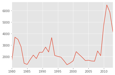
pandas automatically populated the x-axis with the index values (years), and the y-axis with the column values (population). However, notice how the years were not displayed because they are of type string. Therefore, let’s change the type of the index values to integer for plotting.

Also, let’s label the x and y axis using plt.title(), plt.ylabel(), and plt.xlabel() as follows:

haiti.index = haiti.index.map(int) # let's change the index values of Haiti to type integer for plotting
haiti.plot(kind='line')

plt.title('Immigration from Haiti')
plt.ylabel('Number of immigrants')
plt.xlabel('Years')

plt.show() # need this line to show the updates made to the figure

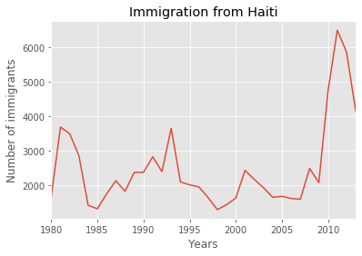
We can clearly notice how number of immigrants from Haiti spiked up from 2010 as Canada stepped up its efforts to accept refugees from Haiti. Let’s annotate this spike in the plot by using the plt.text() method.

haiti.plot(kind='line')

plt.title('Immigration from Haiti')
plt.ylabel('Number of Immigrants')
plt.xlabel('Years')

# annotate the 2010 Earthquake.
# syntax: plt.text(x, y, label)
plt.text(2000, 6000, '2010 Earthquake') # see note below

plt.show()

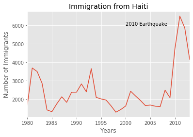
With just a few lines of code, you were able to quickly identify and visualize the spike in immigration!

Quick note on x and y values in plt.text(x, y, label):

 Since the x-axis (years) is type 'integer', we specified x as a year. The y axis (number of immigrants) is type 'integer', so we can just specify the value y = 6000.

    plt.text(2000, 6000, '2010 Earthquake') # years stored as type int

If the years were stored as type 'string', we would need to specify x as the index position of the year. Eg 20th index is year 2000 since it is the 20th year with a base year of 1980.

    plt.text(20, 6000, '2010 Earthquake') # years stored as type int

We will cover advanced annotation methods in later modules.

We can easily add more countries to line plot to make meaningful comparisons immigration from different countries.

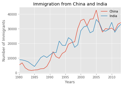
Question: Let’s compare the number of immigrants from India and China from 1980 to 2013.

Step 1: Get the data set for China and India, and display dataframe.

### type your answer here
df_CI = df_can.loc[['China','India'], years]
df_CI

	1980	1981	1982	1983	1984	1985	1986	1987	1988	1989	...	2004	2005	2006	2007	2008	2009	2010	2011	2012	2013
China	5123	6682	3308	1863	1527	1816	1960	2643	2758	4323	...	36619	42584	33518	27642	30037	29622	30391	28502	33024	34129
India	8880	8670	8147	7338	5704	4211	7150	10189	11522	10343	...	28235	36210	33848	28742	28261	29456	34235	27509	30933	33087

2 rows × 34 columns

Double-click here for the solution.

Step 2: Plot graph. We will explicitly specify line plot by passing in kind parameter to plot().

### type your answer here

df_CI.plot(kind='line')

<matplotlib.axes._subplots.AxesSubplot at 0x190036b3470>

Double-click here for the solution.

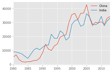
That doesn’t look right…

Recall that pandas plots the indices on the x-axis and the columns as individual lines on the y-axis. Since df_CI is a dataframe with the country as the index and years as the columns, we must first transpose the dataframe using transpose() method to swap the row and columns.

df_CI = df_CI.transpose()
df_CI.head()

pandas will auomatically graph the two countries on the same graph. Go ahead and plot the new transposed dataframe. Make sure to add a title to the plot and label the axes.

### type your answer here
df_CI.plot(kind='line')

plt.title('Immigration from China and India')
plt.ylabel('Number of Immigrants')
plt.xlabel('Years')

Text(0.5, 0, 'Years')

Double-click here for the solution.

From the above plot, we can observe that the China and India have very similar immigration trends through the years.

Note: How come we didn’t need to transpose Haiti’s dataframe before plotting (like we did for df_CI)?

That’s because haiti is a series as opposed to a dataframe, and has the years as its indices as shown below.

print(type(haiti))
print(haiti.head(5))

class ‘pandas.core.series.Series’

1980 1666

1981 3692

1982 3498

1983 2860

1984 1418

Name: Haiti, dtype: int64

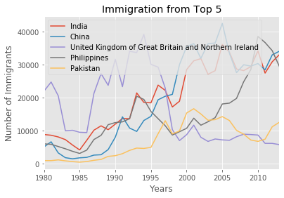
Line plot is a handy tool to display several dependent variables against one independent variable. However, it is recommended that no more than 5-10 lines on a single graph; any more than that and it becomes difficult to interpret.

Question: Compare the trend of top 5 countries that contributed the most to immigration to Canada.

### type your answer here
df_5 = df_can.sort_values(by='Total', ascending = False).head(5).loc[:,years]
df_5 = df_5.T
df_5.plot(kind='line')

plt.title('Immigration from Top 5')
plt.ylabel('Number of Immigrants')
plt.xlabel('Years')

Text(0.5, 0, 'Years')

Double-click here for the solution.

Other Plots

Congratulations! you have learned how to wrangle data with python and create a line plot with Matplotlib. There are many other plotting styles available other than the default Line plot, all of which can be accessed by passing kind keyword to plot(). The full list of available plots are as follows:

• bar for vertical bar plots
• barh for horizontal bar plots
• hist for histogram
• box for boxplot
• kde or density for density plots
• area for area plots
• pie for pie plots
• scatter for scatter plots
• hexbin for hexbin plot

This notebook is part of a course on Coursera called Data Visualization with Python. If you accessed this notebook outside the course, you can take this course online by clicking here.

---

Copyright © 2019 Cognitive Class. This notebook and its source code are released under the terms of the MIT License.