Environment: Python3.7
01. Import the packages
Basic Packages
## import pandas as pd
import geopandas as gpd
import numpy as np
import pandas as pd
import matplotlib.pyplot  as plt
from shapely.geometry import Point #turn latitude and longtitude into geographic points on the global
%matplotlib inline
from shapely.geometry import Polygon
Geocoder packages
from geopy.geocoders import Nominatim
from geopy.geocoders import GoogleV3
02. Importing shp files
Shapefile contents
shp file is not one file, it includes several files with the same name but different file types.
Geopandas is made based on pandas, so the ways to read files are similar.
But no matter what kind of file we are reading in Geopandas, we use gpd.read_file.
cities = gpd.read_file('D:\ARCGIS\Covid-19 Cases in New Zealand\output\DHI_POINTS.shp')
cities.head(2)
| OBJECTID_1 | OBJECTID | DHB2015_Co | DHB2015_Na | Shape_Leng | Shape_Le_1 | ORIG_FID | geometry | |
|---|---|---|---|---|---|---|---|---|
| 0 | 1 | 100 | 01 | Northland | 1.651929e+06 | 16.524423 | 0 | POINT (173.82591 -35.48993) |
| 1 | 2 | 100 | 02 | Waitemata | 9.273920e+05 | 9.301324 | 1 | POINT (174.54665 -36.56396) |
The last column is the geometry of the shp file data.
The geometry includes: Point, Line, Ploygon
Plot the shp files
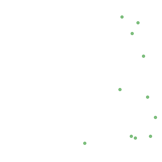
cities.plot()
<matplotlib.axes._subplots.AxesSubplot at 0x1d7968f8e48>
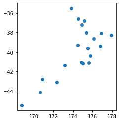
Districts = gpd.read_file(r'D:\ARCGIS\mygeodata\nz_ta-polygon.shp')
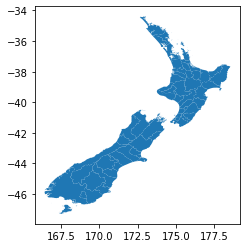
Districts.plot()
<matplotlib.axes._subplots.AxesSubplot at 0x1d794570be0>
Districts.head(5)
| TA2016 | TA2016_NAM | AREA_SQ_KM | LAND_SQ_KM | rmapshaper | geometry | |
|---|---|---|---|---|---|---|
| 0 | 001 | Far North District | 6689.8397 | 6677.4102 | 0 | MULTIPOLYGON (((173.57980 -35.35020, 173.58690... |
| 1 | 002 | Whangarei District | 2711.7983 | 2711.7983 | 1 | MULTIPOLYGON (((174.70210 -35.95510, 174.71330... |
| 2 | 003 | Kaipara District | 3108.7123 | 3108.7123 | 2 | POLYGON ((173.76480 -35.60640, 173.75930 -35.6... |
| 3 | 011 | Thames-Coromandel District | 2207.0122 | 2207.0122 | 3 | MULTIPOLYGON (((175.92670 -37.06880, 175.92890... |
| 4 | 012 | Hauraki District | 1270.0486 | 1270.0486 | 4 | MULTIPOLYGON (((175.54000 -37.16870, 175.54210... |
Data Selection and treatment
Data selection and munipulation in Geopandas is same as Pandas, so it would be easy for those who are familiar with Pandas Packages.
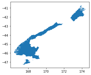
Select the District with the area over 10000
Districts[Districts.AREA_SQ_KM > 10000]
| TA2016 | TA2016_NAM | AREA_SQ_KM | LAND_SQ_KM | rmapshaper | geometry | |
|---|---|---|---|---|---|---|
| 44 | 053 | Marlborough District | 10470.4614 | 10457.6710 | 44 | MULTIPOLYGON (((174.10160 -41.53220, 174.10220... |
| 48 | 057 | Westland District | 11862.7155 | 11827.8208 | 48 | MULTIPOLYGON (((170.18810 -43.21380, 170.18780... |
| 62 | 073 | Southland District | 30198.4023 | 29552.3318 | 62 | MULTIPOLYGON (((167.39580 -47.26400, 167.39830... |
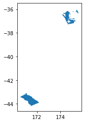
Districts[Districts.AREA_SQ_KM > 10000].plot()
<matplotlib.axes._subplots.AxesSubplot at 0x1d7985a87b8>
Select the District with the name starting with ‘A’
Districts[Districts.TA2016_NAM.str.startswith('A')]
| TA2016 | TA2016_NAM | AREA_SQ_KM | LAND_SQ_KM | rmapshaper | geometry | |
|---|---|---|---|---|---|---|
| 53 | 063 | Ashburton District | 6189.5196 | 6182.5534 | 53 | POLYGON ((172.19490 -43.90370, 172.18710 -43.9... |
| 65 | 076 | Auckland | 4940.8756 | 4939.8049 | 65 | MULTIPOLYGON (((175.16600 -36.90360, 175.16900... |
Districts[Districts.TA2016_NAM.str.startswith('A')].plot()
<matplotlib.axes._subplots.AxesSubplot at 0x1d7985d5c50>
Write the info into files
Writing to shp files
cities.to_file('D:\ARCGIS\Covid-19 Cases in New Zealand\output\DHI_POINTS_COPY.shp')
Writing to GeoJason
cities.to_file('D:\ARCGIS\Covid-19 Cases in New Zealand\output\DHI_POINTS.geojson', driver = 'GeoJSON')
03. Opening CSV files with geopandas
- open up the csv with pandas
- We’ll take lat/lon feed it to shapely, which creates a Point
- we will use original dataframe and geometry infomation to make geodataframe for Geopandas
- tell the new geodataframe that coords are latitude and longitude
read out the csv files
df = pd.read_csv('Chicago_Public_Schools_-_Progress_Report_Cards__2011-2012-v3.csv')
df.head(2)
| School ID | NAME_OF_SCHOOL | Elementary, Middle, or High School | Street Address | City | State | ZIP Code | Phone Number | Link | Network Manager | ... | Freshman on Track Rate % | X_COORDINATE | Y_COORDINATE | Latitude | Longitude | COMMUNITY_AREA_NUMBER | COMMUNITY_AREA_NAME | Ward | Police District | Location | |
|---|---|---|---|---|---|---|---|---|---|---|---|---|---|---|---|---|---|---|---|---|---|
| 0 | 610038 | Abraham Lincoln Elementary School | ES | 615 W Kemper Pl | Chicago | IL | 60614 | (773) 534-5720 | http://schoolreports.cps.edu/SchoolProgressRep... | Fullerton Elementary Network | ... | NDA | 1171699.458 | 1915829.428 | 41.924497 | -87.644522 | 7 | LINCOLN PARK | 43 | 18 | (41.92449696, -87.64452163) |
| 1 | 610281 | Adam Clayton Powell Paideia Community Academy ... | ES | 7511 S South Shore Dr | Chicago | IL | 60649 | (773) 535-6650 | http://schoolreports.cps.edu/SchoolProgressRep... | Skyway Elementary Network | ... | NDA | 1196129.985 | 1856209.466 | 41.760324 | -87.556736 | 43 | SOUTH SHORE | 7 | 4 | (41.76032435, -87.55673627) |
2 rows × 78 columns
Select the column data we need
df2 = df.loc[:,['NAME_OF_SCHOOL','City','Latitude','Longitude' ]]
df2.head()
| NAME_OF_SCHOOL | City | Latitude | Longitude | |
|---|---|---|---|---|
| 0 | Abraham Lincoln Elementary School | Chicago | 41.924497 | -87.644522 |
| 1 | Adam Clayton Powell Paideia Community Academy ... | Chicago | 41.760324 | -87.556736 |
| 2 | Adlai E Stevenson Elementary School | Chicago | 41.747111 | -87.731702 |
| 3 | Agustin Lara Elementary Academy | Chicago | 41.809757 | -87.672145 |
| 4 | Air Force Academy High School | Chicago | 41.828146 | -87.632794 |
Point(-78,40)
Creating shapely Points from latitude and longtitude
points = df2.apply(lambda row:Point(row.Longitude,row.Latitude), axis =1)# Attention: axis =1
points.head()
0    POINT (-87.64452163 41.92449696)
1    POINT (-87.55673627 41.76032435)
2    POINT (-87.73170248 41.74711093)
3      POINT (-87.6721446 41.8097569)
4    POINT (-87.63279369 41.82814609)
dtype: object
Making a geodataframe by dataframe and geo point information
schools = gpd.GeoDataFrame(df2,geometry = points)
schools.crs = {'init':'epsg:4326'}   #project system
schools.head(2)
C:\Python37\lib\site-packages\pyproj\crs\crs.py:53: FutureWarning: '+init=<authority>:<code>' syntax is deprecated. '<authority>:<code>' is the preferred initialization method. When making the change, be mindful of axis order changes: https://pyproj4.github.io/pyproj/stable/gotchas.html#axis-order-changes-in-proj-6
  return _prepare_from_string(" ".join(pjargs))
| NAME_OF_SCHOOL | City | Latitude | Longitude | geometry | |
|---|---|---|---|---|---|
| 0 | Abraham Lincoln Elementary School | Chicago | 41.924497 | -87.644522 | POINT (-87.64452 41.92450) |
| 1 | Adam Clayton Powell Paideia Community Academy ... | Chicago | 41.760324 | -87.556736 | POINT (-87.55674 41.76032) |
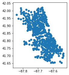
schools.plot()
<matplotlib.axes._subplots.AxesSubplot at 0x1d7967c0390>
04. What is a Coordinate Reference Systems
Ellipsoid - shape of the earth
Datum - where is the ellipsoid goes
http://epsg.io/ to get the EPSG No. for certain address
EPSG standards for European petroleum survey group
WGS84 – EPSG:4326
NAD83 – EPSG:4269
GDA94 – EPSG:4939
IAU codes
05. Customizing map projections in geopandas
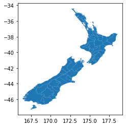
Districts.plot()
<matplotlib.axes._subplots.AxesSubplot at 0x1d796447e80>
Districts.to_crs({'proj':'merc'}).plot(figsize = (10,10))
<matplotlib.axes._subplots.AxesSubplot at 0x1d79605efd0>
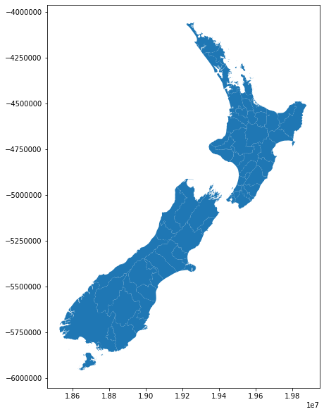
We can see although the shape is still similar, the X,Y axes are different since the coordinate system has changed.
06. Customizing basic map styles with geopandas
pass parameter to .plot
work with the ax variable
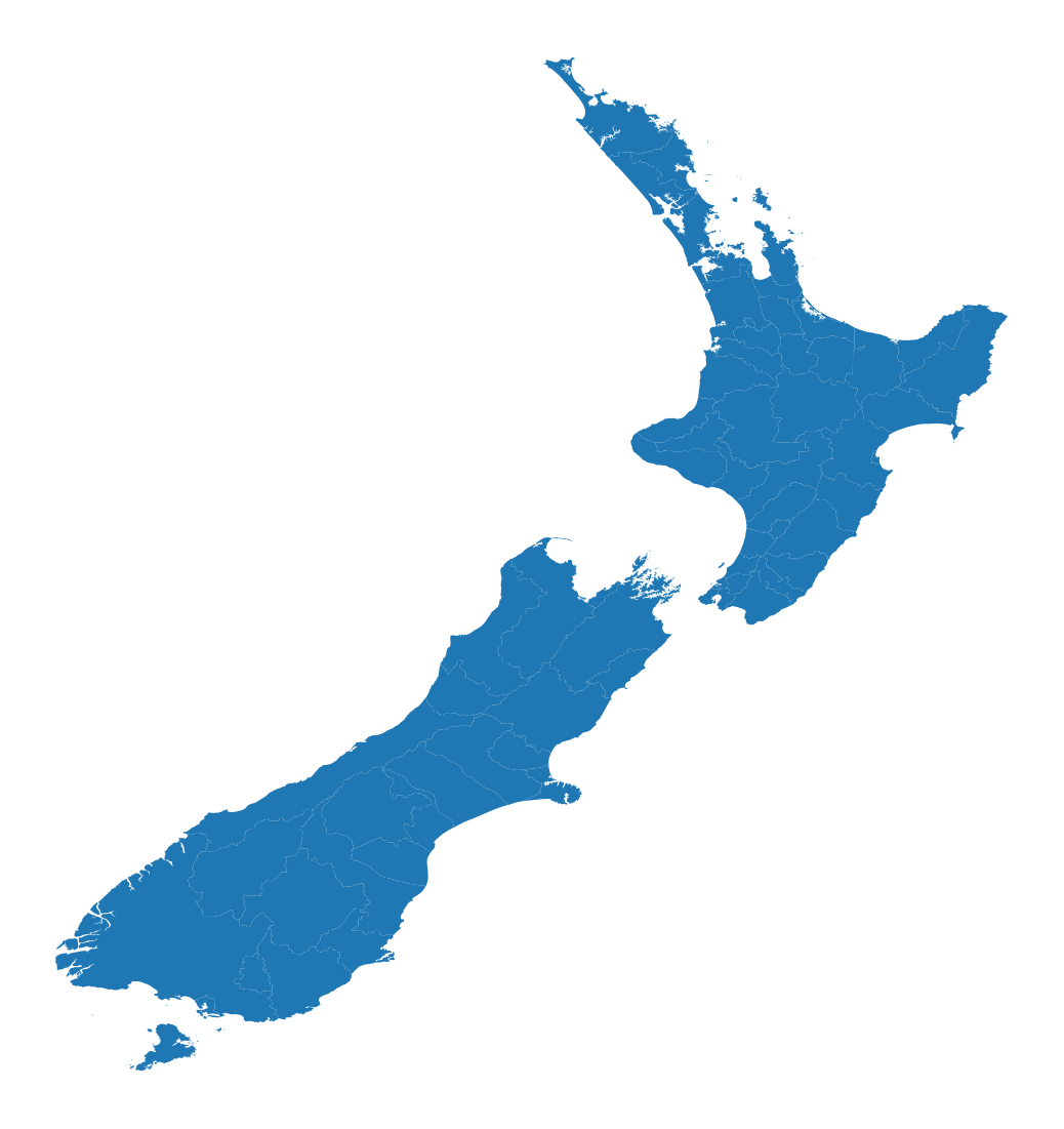
ax = Districts.plot(figsize = (20,20))
ax.axis('off')
(165.81877500000002, 179.184325, -47.934870000000004, -33.747730000000004)
coloring shape
1.fill - inside part
2. strike/line/edge - outline
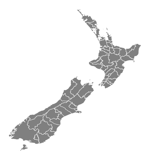
ax = Districts.plot(figsize = (10,10), color = 'grey', edgecolor = 'white')
ax.axis('off')
(165.81877500000002, 179.184325, -47.934870000000004, -33.747730000000004)
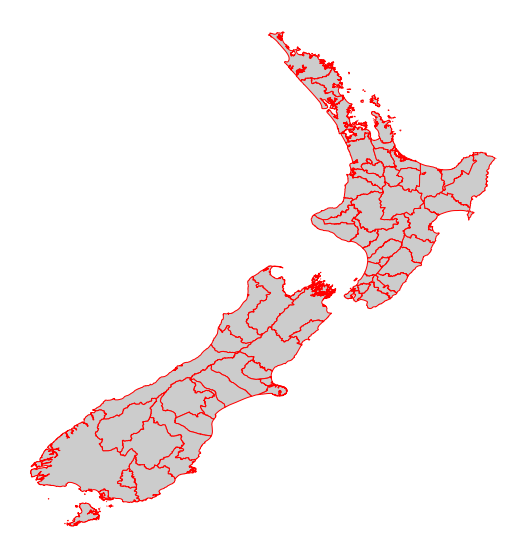
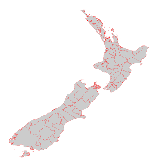
ax = Districts.plot(figsize = (10,10), color = '#CCCCCC', edgecolor = '#FF0000')
ax.axis('off')
(165.81877500000002, 179.184325, -47.934870000000004, -33.747730000000004)
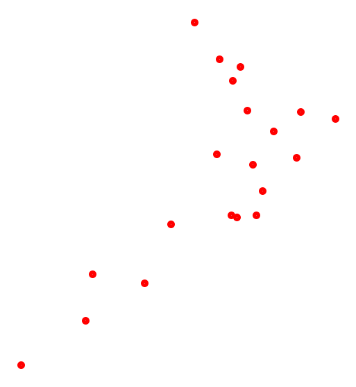
ax = cities.plot(figsize = (10,10), color = '#CCCCCC', edgecolor = '#FF0000', linewidth = 5)
ax.axis('off')
(168.32748359957623,
 178.38357246311102,
 -45.94570795960331,
 -34.986255336266005)
ax = Districts.plot(figsize = (10,10), color = '#CCCCCC', edgecolor = '#FF0000', linewidth = 0.25)
ax.axis('off')
(165.81877500000002, 179.184325, -47.934870000000004, -33.747730000000004)
Districts.head()
| TA2016 | TA2016_NAM | AREA_SQ_KM | LAND_SQ_KM | rmapshaper | geometry | |
|---|---|---|---|---|---|---|
| 0 | 001 | Far North District | 6689.8397 | 6677.4102 | 0 | MULTIPOLYGON (((173.57980 -35.35020, 173.58690... |
| 1 | 002 | Whangarei District | 2711.7983 | 2711.7983 | 1 | MULTIPOLYGON (((174.70210 -35.95510, 174.71330... |
| 2 | 003 | Kaipara District | 3108.7123 | 3108.7123 | 2 | POLYGON ((173.76480 -35.60640, 173.75930 -35.6... |
| 3 | 011 | Thames-Coromandel District | 2207.0122 | 2207.0122 | 3 | MULTIPOLYGON (((175.92670 -37.06880, 175.92890... |
| 4 | 012 | Hauraki District | 1270.0486 | 1270.0486 | 4 | MULTIPOLYGON (((175.54000 -37.16870, 175.54210... |
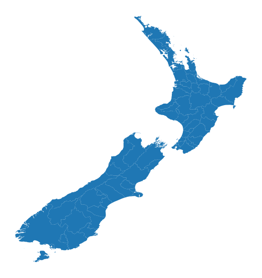
ax = Districts.plot(figsize = (10,10))
ax.axis('off')
(165.81877500000002, 179.184325, -47.934870000000004, -33.747730000000004)
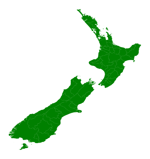
ax = Districts.plot(figsize = (10,10), color = 'green')
ax.axis('off')
(165.81877500000002, 179.184325, -47.934870000000004, -33.747730000000004)
ax = Districts.plot(figsize = (10,10), color = 'green',  markersize =100 ,alpha =0.5)
ax.axis('off')
(165.81877500000002, 179.184325, -47.934870000000004, -33.747730000000004)
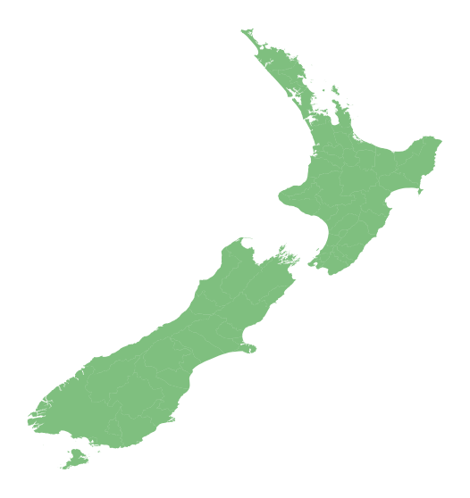
ax = cities.plot(figsize = (10,10), color = 'green', markersize =100 ,alpha =0.5)
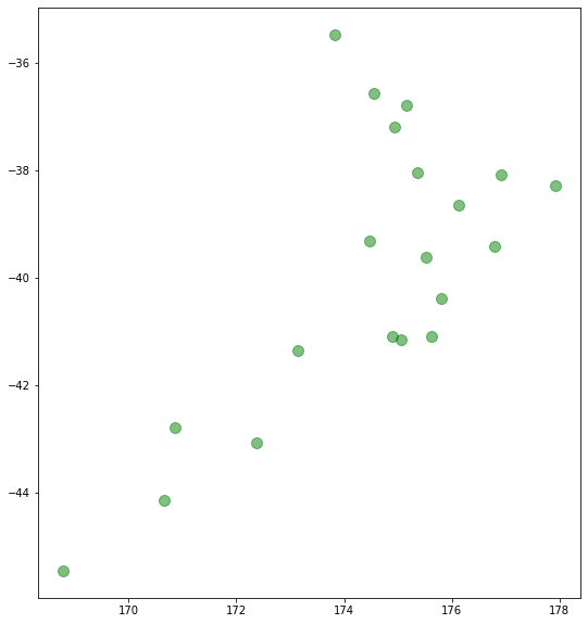
ax = cities.plot(figsize = (10,10), color = 'green',  markersize =100 ,alpha =0.5)
ax.axis('off')
ax.set_xlim([170,176])
ax.set_ylim([-42,-36])
(-42, -36)